IA modelling, step by step · Sinusoidal

Sinusoidal model, step by step: y = a sin(b(x − c)) + d

AA SLAA HLAI SLAI HL

For anything that repeats — daylight, tides, temperatures, a Ferris wheel — find a, b, c and d by hand from the maximum, minimum and period, convert to the calculator's form a sin(bx + c) + d, then refine the fit by minimising the sum of squared residuals.

Guidance based on the checklist Pete Bromfield — an IB examiner and former Head of Maths — uses with his own students. Not affiliated with or endorsed by the IB.

Example data, invented for this guide. The context is realistic, but the numbers were made up to show the method. Use your own measured or sourced data in your IA.

When to use it

The shape of the data

The data rise and fall repeatedly, with peaks the same height and troughs the same depth.
Peaks (and troughs) are equally spaced: a fixed period.
The curve is symmetric about a middle line.

The context

Anything driven by the Earth's rotation or orbit: daylight, temperature, tides.
Rotations: a Ferris wheel seat, a point on a bicycle wheel.
Seasonal sales or visitor numbers (check that the peaks really are equal).

Course fit: AA SL and HL use y = a sin(b(x + c)) + d; AI SL uses a sin(bx) + d and AI HL adds the horizontal shift and sine regression. Whatever your course, show the by-hand estimates and explain the refinement.

The example data

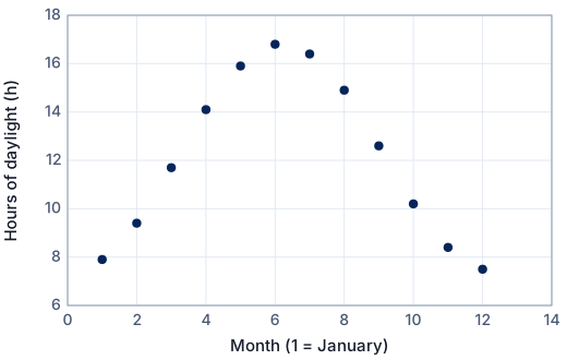
Hours of daylight on the 15th of each month for a city at about 52° N, read from a sunrise–sunset table (values rounded to 0.1 h and slightly perturbed for this example).

Example data: hours of daylight and month (1 = january)
i	x: Month (1 = January)	y: Hours of daylight (h)
1	1	7.9
2	2	9.4
3	3	11.7
4	4	14.1
5	5	15.9
6	6	16.8
7	7	16.4
8	8	14.9
9	9	12.6
10	10	10.2
11	11	8.4
12	12	7.5

Scatter graph of hours of daylight against month (1 = january) for the example data — Step 1 of any modelling IA: plot the data and describe the shape before fitting anything.

The method: estimate by hand, then refine

Steps 1–6 find each parameter from the graph, using the known period of 12 months. Steps 7–8 then let all four parameters vary to minimise the sum of squared residuals, which is what sine regression does.

Step 1 · Read the maximum and minimum

Highest point: y_max = 16.8 at x = 6. Lowest point: y_min = 7.5 at x = 12.

Step 2 · Amplitude a and principal axis d

a = (y_max − y_min)/2 = (16.8 − 7.5)/2 = 4.650

d = (y_max + y_min)/2 = (16.8 + 7.5)/2 = 12.15

The principal axis y = d is the middle of the oscillation; a is the distance from it to a peak.

Step 3 · Period and b

From the context, one full cycle takes P = 12.

b = 2π/P = 2π/12 = 0.5236 radians per unit of x

In degree mode the same curve has b = 360°/P = 30.00° per unit. Use one angle mode throughout: GDC sine regression expects radians.

Step 4 · Horizontal shift c

y = a sin(b(x − c)) + d has a maximum where b(x − c) = π/2, i.e. a quarter-period after x = c. Put that maximum at x = 6:

c = x_max − P/4 = 6 − 12/4 = 3.000

Equivalently, c is where the curve crosses the principal axis going up.

Step 5 · The first model, in both forms

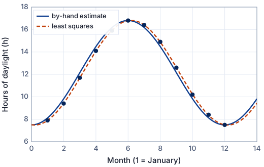
y = 4.650 sin(0.5236(x − 3.000)) + 12.15

Expanding the bracket, b(x − c) = bx − bc, so the form y = a sin(bx + C) + d (the one GDCs use) has C = −bc = −0.5236 × 3.000 = −1.571:

y = 4.650 sin(0.5236x − 1.571) + 12.15

Step 6 · How well does the first model fit?

For each point, the residual is the observed value minus the model's value: e = y − ŷ.

Residuals
i	x	y (data)	ŷ (model)	y − ŷ	(y − ŷ)²
1	1	7.9	8.123	−0.223	0.0497
2	2	9.4	9.825	−0.425	0.181
3	3	11.7	12.15	−0.450	0.203
4	4	14.1	14.47	−0.375	0.141
5	5	15.9	16.18	−0.277	0.0767
6	6	16.8	16.80	0.00	0.00
7	7	16.4	16.18	0.223	0.0497
8	8	14.9	14.48	0.425	0.181
9	9	12.6	12.15	0.450	0.202
10	10	10.2	9.825	0.375	0.141
11	11	8.4	8.123	0.277	0.0767
12	12	7.5	7.500	0.00	0.00
Σ					1.300

Sum of squared residuals: SSR = Σ(y − ŷ)² = 1.300
Total sum of squares about the mean ȳ = 12.15: SST = Σ(y − ȳ)² = 130.6
Coefficient of determination: R² = 1 − SSR/SST = 1 − 1.300/130.6 = 0.9900
Root-mean-square error: RMSE = √(SSR/n) = 0.329 — a typical size of a residual, in the units of y.

Step 7 · Refine: minimise the sum of squared residuals

The estimates came from only two points. Least squares adjusts all four parameters together until SSR is as small as possible. There is no formula for this: it is done iteratively (the Gauss–Newton / Levenberg–Marquardt method, which is what a GDC's sine regression and Desmos do), starting from the estimates above.

y = 4.665 sin(0.5238(x − 3.191)) + 12.15

y = 4.665 sin(0.5238x − 1.671) + 12.15 (C = −bc)

That is a = 4.665, b = 0.5238, c = 3.191, d = 12.15, with period P = 2π/b = 12.00. A calculator may show an equivalent answer: adding 2π to C, or changing the sign of a and shifting c by half a period, gives the same curve.

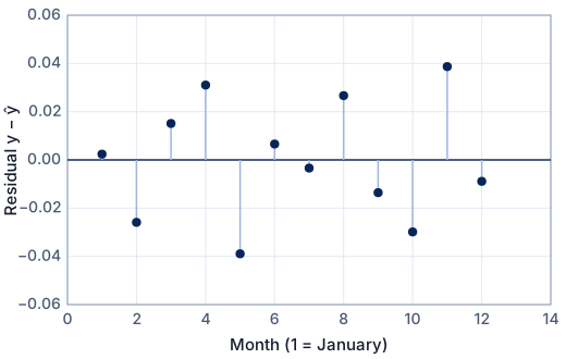
Step 8 · Residuals of the refined model

For each point, the residual is the observed value minus the model's value: e = y − ŷ.

Residuals
i	x	y (data)	ŷ (model)	y − ŷ	(y − ŷ)²
1	1	7.9	7.898	0.00240	0.00000577
2	2	9.4	9.426	−0.0259	0.000670
3	3	11.7	11.68	0.0151	0.000228
4	4	14.1	14.07	0.0310	0.000964
5	5	15.9	15.94	−0.0389	0.00151
6	6	16.8	16.79	0.00659	0.0000434
7	7	16.4	16.40	−0.00337	0.0000113
8	8	14.9	14.87	0.0267	0.000710
9	9	12.6	12.61	−0.0136	0.000184
10	10	10.2	10.23	−0.0299	0.000891
11	11	8.4	8.361	0.0387	0.00150
12	12	7.5	7.509	−0.00890	0.0000791
Σ					0.006798

Sum of squared residuals: SSR = Σ(y − ŷ)² = 0.006798
Total sum of squares about the mean ȳ = 12.15: SST = Σ(y − ȳ)² = 130.6
Coefficient of determination: R² = 1 − SSR/SST = 1 − 0.006798/130.6 = 0.9999
Root-mean-square error: RMSE = √(SSR/n) = 0.0238 — a typical size of a residual, in the units of y.

SSR fell from 1.300 to 0.006798.

Graph of the data with the fitted sinusoidal (by-hand estimate) — Estimate by hand, then refine: the fitted curves over the example data.

Residual plot for the sinusoidal fitted to the example data — Residuals against x. Look for a pattern: random scatter about 0 means the model has captured the shape; a curve or a trend means it has not.

What the model tells you

a ≈ 4.67 h: the longest day is about 4.7 hours longer than the average day, and the shortest about 4.7 hours shorter.
d ≈ 12.15 h: the average day length is about 12 hours, as it must be over a year (days and nights balance out).
The refined period is 12.00 months, almost exactly the 12 months the context predicts. If you know the period exactly, it is reasonable to fix it and fit only a, c and d — say which you did.
c ≈ 3.19: the curve crosses its principal axis going up at month 3.19, close to the March equinox (month 3 is mid-March in this data, because each reading is on the 15th).

The same on a GDC

Enter and plot the data first, then fit. The key sequences are for current operating systems; menus differ slightly between versions.

TI-84 Plus CE

Data: [stat] → 1: Edit… Type the x values in L1 and the y values in L2. To plot: [2nd] [y=] (STAT PLOT) → Plot1: On, Type: scatter, Xlist: L1, Ylist: L2, then [zoom] → 9: ZoomStat.
Set radians first: [mode] → RADIAN.
[stat] → CALC → C: SinReg. Xlist: L1, Ylist: L2, Period: 12 (optional but it helps), Store RegEQ: Y1. Calculate.
It fits y = a·sin(bx + c) + d — the calculator's c is our C = −bc.
Residuals are in the list RESID, as for any regression.

TI-Nspire CX

Data: Add a Lists & Spreadsheet page; name column A xs and column B ys and type the data. Add a Data & Statistics page (or a Graphs page with menu → Graph Entry/Edit → Scatter Plot) and choose xs and ys.
Set the document to radians (the angle mode in the document settings).
menu → Statistics → Stat Calculations → Sinusoidal Regression, X List xs, Y List ys; give a period if you know it; save to f1.
Result: y = a·sin(bx + c) + d.

Casio fx-CG50

Data: [MENU] → Statistics. Type the x values in List 1 and the y values in List 2. To plot: [F1] (GRAPH) → [F6] (SET): Graph Type Scatter, XList List1, YList List2; [EXIT], then [F1] (GRAPH1).
[SHIFT] [MENU] (SET UP) → Angle: Rad.
Statistics → [F2] (CALC) → [F3] (REG) → [F6] (▷) → [F4] (Sin). Shows a, b, c, d for y = a·sin(bx + c) + d.
[F5] (COPY) to draw it over the scatter plot.

In Desmos

Free at desmos.com/calculator. In a regression, ~ means “fit this model”; subscripts are typed with an underscore (x_1 shows as x₁).

Data in x₁, y₁ (Desmos works in radians by default — check the wrench menu).
Type y_1 ~ a sin(b x_1 + c) + d.
If the fit looks wrong, Desmos started from a poor guess. Fix b from the period you know: y_1 ~ a sin(π/6 (x_1 - c)) + d, or give the parameters starting values with sliders first.
Compare with your by-hand model by typing it as y = 4.650 sin(0.5236(x - 3.000)) + 12.15.

More on technology in the IA: using Desmos, GeoGebra and Excel.

How to write it up in your IA

Say why a periodic model suits the context and what the period should be before looking at the data.
Find a, d, b and c from the graph with each step explained — this is the mathematics the examiner wants to see.
Show the link between the two forms: a sin(b(x − c)) + d and a sin(bx + C) + d with C = −bc.
State the angle mode (radians) and why it matters.
Compare the by-hand model with the refined one using SSR, and say what refinement does and why it lowers SSR.
Interpret each parameter in context and state the domain; discuss whether the pattern repeats exactly year to year.

These are the points to cover, not sentences to copy. Write every explanation in your own words, about your own data.

Common mistakes

Degree mode on the GDC: sine regression gives nonsense or will not converge.
Mixing the two forms: a calculator's c is not the horizontal shift; the shift is −c/b.
Estimating the period from two adjacent peaks that are not a full cycle apart.
Using a sine model for data that are not periodic (for example, one rise and fall).
Quoting four parameters to 6 s.f. from eight data points: give sensible accuracy.

Is this good enough for Criterion E?

The period is justified from the context and the graph.
a, b, c and d are each found by hand, with the reasoning written in words.
The conversion between the two forms is shown and consistent.
The refined (regression) model is compared with the by-hand model using SSR or R².
Parameters are interpreted in context; limitations of assuming exact periodicity are discussed.
HL: the refinement is explained (minimising SSR iteratively), or the model is extended (for example, a sum of two sine terms, or a varying amplitude).

SL or HL? Criterion E asks for mathematics that fits your course. At SL, fitting with technology is fine when you explain the method and justify every choice. At HL, show more of the mathematics yourself — the last item in the list is an example. See Criterion E and Criterion D.

Frequently asked questions

How do I convert a sin(b(x − c)) + d into a sin(bx + c) + d?

Expand the bracket: b(x − c) = bx − bc. So the calculator's constant is C = −bc, and the horizontal shift is c = −C/b.

Why does my calculator give a negative a for a sine model?

Different parameter sets can draw the same curve: changing the sign of a and shifting by half a period, or adding 2π to the constant, gives an identical graph. Convert to your preferred form and say so.

Free: the IA checklist an examiner uses

Every check for Criteria A–E in a 4-page PDF, the mistakes that cost the most marks and a self-assessment grid. We'll email it with a short IA tip every few days, timed to your deadline if you give it. Free — no account, no payment.

Get the free checklist