IA modelling, step by step · Straight line
Straight-line model, step by step: from two points to least squares
A line is the simplest model and the one to beat. Here it is fitted twice to the same data — by hand through two points, then by least squares with every sum shown — followed by r, r² and the residuals, and how to write it up.
Example data, invented for this guide. The context is realistic, but the numbers were made up to show the method. Use your own measured or sourced data in your IA.
When to use it
The shape of the data
- The points lie close to a straight line with no bend.
- Equal steps in x give roughly equal steps in y (constant rate of change).
- The residuals from a line show no pattern.
The context
- A constant rate: cost per item, energy per litre, distance at steady speed.
- Theory predicts proportionality (a line through the origin) or a fixed start-up amount plus a constant rate.
- Short ranges of something that curves over a longer range (say so, and state the domain).
Course fit: Every course. Linear regression, r and the regression line of y on x are in both AA and AI at SL; in an IA the credit comes from explaining and interpreting them, not from pressing LinReg.
The example data
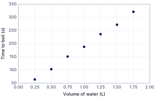
A student times how long a 2.2 kW kettle takes to boil different volumes of tap water, starting from the same tap temperature (about 15 °C) each time.
| i | x: Volume of water (L) | y: Time to boil (s) |
|---|---|---|
| 1 | 0.25 | 64 |
| 2 | 0.5 | 103 |
| 3 | 0.75 | 151 |
| 4 | 1 | 188 |
| 5 | 1.25 | 236 |
| 6 | 1.5 | 272 |
| 7 | 1.75 | 321 |
Method 1: by hand through two points
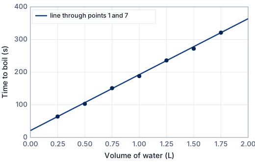
The quickest estimate: draw the line through two points and read off its gradient and intercept. It is a useful first model and a check on the regression, but it ignores the other five points.
Step 1 · Choose two points
Use two points far apart (a wide base reduces the effect of measurement error): point 1 (0.25, 64) and point 7 (1.75, 321).
Step 2 · Gradient
m = (y₂ − y₁)/(x₂ − x₁) = (321 − 64)/(1.75 − 0.25) = 257/1.5 = 171.3
Step 3 · Intercept
c = y₁ − m x₁ = 64 − 171.3 × 0.25 = 21.17
Step 4 · The model
y = 171.3x + 21.17
This line goes exactly through the two chosen points and ignores the others, so it depends on which two you pick. That is why least squares (which uses every point) is the better final model.
Step 5 · Residuals and goodness of fit
For each point, the residual is the observed value minus the model's value: e = y − ŷ.
| i | x | y (data) | ŷ (model) | y − ŷ | (y − ŷ)² |
|---|---|---|---|---|---|
| 1 | 0.25 | 64 | 64.00 | 0.00 | 0.00 |
| 2 | 0.5 | 103 | 106.8 | −3.83 | 14.7 |
| 3 | 0.75 | 151 | 149.7 | 1.33 | 1.78 |
| 4 | 1 | 188 | 192.5 | −4.50 | 20.3 |
| 5 | 1.25 | 236 | 235.3 | 0.667 | 0.444 |
| 6 | 1.5 | 272 | 278.2 | −6.17 | 38.0 |
| 7 | 1.75 | 321 | 321.0 | 0.00 | 0.00 |
| Σ | 75.19 |
- Sum of squared residuals: SSR = Σ(y − ŷ)² = 75.19
- Total sum of squares about the mean ȳ = 190.7: SST = Σ(y − ȳ)² = 50970
- Coefficient of determination: R² = 1 − SSR/SST = 1 − 75.19/50970 = 0.9985
- Root-mean-square error: RMSE = √(SSR/n) = 3.28 — a typical size of a residual, in the units of y.
Method 2: least-squares regression
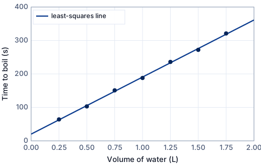
Least squares chooses the line that makes the sum of squared residuals as small as possible. For a line there is an exact formula, and every sum in it can be tabulated — this is what LinReg does.
Step 1 · Tabulate the sums
| i | x | y | x² | xy | y² |
|---|---|---|---|---|---|
| 1 | 0.25 | 64 | 0.0625 | 16 | 4096 |
| 2 | 0.5 | 103 | 0.25 | 51.5 | 10609 |
| 3 | 0.75 | 151 | 0.5625 | 113.25 | 22801 |
| 4 | 1 | 188 | 1 | 188 | 35344 |
| 5 | 1.25 | 236 | 1.5625 | 295 | 55696 |
| 6 | 1.5 | 272 | 2.25 | 408 | 73984 |
| 7 | 1.75 | 321 | 3.0625 | 561.75 | 103041 |
| Σ | 7 | 1335 | 8.75 | 1633.5 | 305571 |
n = 7 points.
Step 2 · Gradient
m = (nΣXY − ΣX ΣY) / (nΣX² − (ΣX)²)
m = (7 × 1633.5 − 7 × 1335) / (7 × 8.75 − 7²) = 2089.5 / 12.25 = 170.6
Here X = x and Y = y.
Step 3 · Intercept
X̄ = ΣX/n = 1.0000, Ȳ = ΣY/n = 190.71
c = Ȳ − m X̄ = 190.71 − 170.6 × 1.0000 = 20.14
The line of best fit always passes through the mean point (X̄, Ȳ).
Step 4 · Correlation
r = (nΣXY − ΣX ΣY) / √[(nΣX² − (ΣX)²)(nΣY² − (ΣY)²)] = 2089.5 / √(12.25 × 356772) = 0.9995
r² = 0.9990: a very strong positive linear correlation between x and y.
Step 5 · The model
y = 170.6x + 20.14
The gradient 170.6 is the change in y for each 1 unit increase in x; the intercept 20.14 is the model's value of y at x = 0 — say whether that means anything in your context.
Step 6 · Residuals and goodness of fit
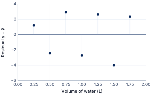
For each point, the residual is the observed value minus the model's value: e = y − ŷ.
| i | x | y (data) | ŷ (model) | y − ŷ | (y − ŷ)² |
|---|---|---|---|---|---|
| 1 | 0.25 | 64 | 62.79 | 1.21 | 1.47 |
| 2 | 0.5 | 103 | 105.4 | −2.43 | 5.90 |
| 3 | 0.75 | 151 | 148.1 | 2.93 | 8.58 |
| 4 | 1 | 188 | 190.7 | −2.71 | 7.37 |
| 5 | 1.25 | 236 | 233.4 | 2.64 | 6.98 |
| 6 | 1.5 | 272 | 276.0 | −4.00 | 16.0 |
| 7 | 1.75 | 321 | 318.6 | 2.36 | 5.56 |
| Σ | 51.86 |
- Sum of squared residuals: SSR = Σ(y − ŷ)² = 51.86
- Total sum of squares about the mean ȳ = 190.7: SST = Σ(y − ȳ)² = 50970
- Coefficient of determination: R² = 1 − SSR/SST = 1 − 51.86/50970 = 0.9990
- Root-mean-square error: RMSE = √(SSR/n) = 2.72 — a typical size of a residual, in the units of y.
For a least-squares line, R² equals r² (0.9990).
What the model tells you
- Gradient ≈ 171 s per litre: each extra litre adds about that many seconds. Compare it with theory: heating 1 kg of water from 15 °C to 100 °C needs 4.186 × 85 ≈ 356 kJ, which a 2.2 kW element supplies in about 162 s. The measured gradient is a little higher, because some energy heats the kettle and the air.
- Intercept ≈ 20.1 s: the time the kettle takes even for a tiny volume (heating the element and the kettle body). It is an extrapolation to x = 0, outside the data, so treat it as an estimate.
- Using the model: 1.2 L should take about 225 s — an interpolation, inside the data, so it is reliable to within a typical residual (RMSE 2.72 s).
- Domain: 0.25 L ≤ x ≤ 1.75 L. Kettles hold at most about 1.7 L, so predictions far beyond the data are meaningless.
The same on a GDC
Enter and plot the data first, then fit. The key sequences are for current operating systems; menus differ slightly between versions.
TI-84 Plus CE
- Data: [stat] → 1: Edit… Type the x values in L1 and the y values in L2. To plot: [2nd] [y=] (STAT PLOT) → Plot1: On, Type: scatter, Xlist: L1, Ylist: L2, then [zoom] → 9: ZoomStat.
- Turn on diagnostics once: [mode] → STAT DIAGNOSTICS: ON (older OS: [2nd] [0] (CATALOG) → DiagnosticOn [enter] [enter]).
- [stat] → CALC → 4: LinReg(ax+b). Xlist: L1, Ylist: L2, Store RegEQ: Y1 ([alpha] [trace] → Y1). Calculate.
- The screen shows a (gradient), b (intercept), r² and r. Note a is the gradient here.
- Residuals: after any regression the list RESID holds them. In L3's header type [2nd] [stat] (LIST) → RESID [enter].
TI-Nspire CX
- Data: Add a Lists & Spreadsheet page; name column A xs and column B ys and type the data. Add a Data & Statistics page (or a Graphs page with menu → Graph Entry/Edit → Scatter Plot) and choose xs and ys.
- menu → Statistics → Stat Calculations → Linear Regression (mx+b). X List: xs, Y List: ys, Save RegEqn to: f1. OK.
- m, b, r² and r appear in the next empty columns, with the residuals as stat.resid.
- Predict with f1(1.2) on a Calculator page.
Casio fx-CG50
- Data: [MENU] → Statistics. Type the x values in List 1 and the y values in List 2. To plot: [F1] (GRAPH) → [F6] (SET): Graph Type Scatter, XList List1, YList List2; [EXIT], then [F1] (GRAPH1).
- [F2] (CALC) → [F6] (SET): 2Var XList List1, 2Var YList List2, 2Var Freq 1. [EXIT].
- [F3] (REG) → [F1] (X) → [F1] (ax+b). The screen shows a (gradient), b (intercept), r, r² and MSe.
- To store residuals: [SHIFT] [MENU] (SET UP) → Resid List → a spare list, then run the regression again.
- [F5] (COPY) pastes the equation into the Graph list so you can draw it over the scatter plot.
In Desmos
Free at desmos.com/calculator. In a regression, ~ means “fit this model”; subscripts are typed with an underscore (x_1 shows as x₁).
- Add a table (+ → table) with the data in x₁ and y₁.
- Type
y_1 ~ m x_1 + c. Desmos shows m, c, r and R² and draws the line. - Tick “plot” next to the residuals e₁ to see the residual plot.
More on technology in the IA: using Desmos, GeoGebra and Excel.
How to write it up in your IA
- Show the scatter graph first and say why a line is a reasonable candidate (shape and context).
- Show one full calculation — the Σ table and the formulas — then say that technology was used for the rest and gives the same result.
- Define every variable with units (x = volume in litres, y = time in seconds) and state the domain.
- Interpret the gradient and intercept in the context, and say whether the intercept is meaningful.
- Quote r and r², and say what they do and do not show (a high r does not prove a line is the right shape — look at the residuals).
- Compare the two-point line with the least-squares line using SSR, and explain why least squares is preferred.
These are the points to cover, not sentences to copy. Write every explanation in your own words, about your own data.
Common mistakes
- Quoting r without a graph: a curve can have r above 0.9.
- Mixing up a and b: on TI and Casio LinReg(ax+b), a is the gradient; on some calculators (a + bx) it is the intercept.
- Rounding the gradient to 2 s.f. before working out the intercept.
- Forcing the line through the origin when the context has a fixed start-up amount.
- Predicting far outside the data range without saying it is an extrapolation.
Is this good enough for Criterion E?
- The scatter graph is shown, labelled, with units.
- The choice of a linear model is justified by the data shape and the context.
- One least-squares calculation is shown in full; technology use is stated.
- Gradient and intercept are interpreted in context, with the domain stated.
- r (or r²) and the residuals are used to judge the fit — not r alone.
- At least one other model or method is compared, and the better one chosen for a reason.
- HL: the least-squares formulas are derived (for example by minimising SSR with calculus) or the uncertainty in the gradient is discussed.
SL or HL? Criterion E asks for mathematics that fits your course. At SL, fitting with technology is fine when you explain the method and justify every choice. At HL, show more of the mathematics yourself — the last item in the list is an example. See Criterion E and Criterion D.
Frequently asked questions
Do I need to calculate the regression line by hand in my IA?
No, but showing one complete calculation (the sums and the formulas) shows understanding, and then technology can do the rest. What earns marks is explaining the method and interpreting the result.
What is the difference between r and r²?
r measures the strength and direction of linear correlation (−1 to 1). r² is the proportion of the variation in y explained by the line. For a least-squares line, r² equals the coefficient of determination R².
Free: the IA checklist an examiner uses
Every check for Criteria A–E in a 4-page PDF, the mistakes that cost the most marks and a self-assessment grid. We'll email it with a short IA tip every few days, timed to your deadline if you give it. Free — no account, no payment.
While you wait for the email: read the full modelling workflow →