IA modelling, step by step · Logistic

Logistic model, step by step: y = L/(1 + C e^(−kx))

AI HL

S-shaped growth — plants, epidemics, app downloads, the spread of news — starts almost exponential and levels off at a ceiling L. Estimate L, linearise to find C and k, then let a least-squares refinement adjust all three.

Guidance based on the checklist Pete Bromfield — an IB examiner and former Head of Maths — uses with his own students. Not affiliated with or endorsed by the IB.

Example data, invented for this guide. The context is realistic, but the numbers were made up to show the method. Use your own measured or sourced data in your IA.

When to use it

The shape of the data

An S-shape: slow start, steep middle, then levelling off.
The fastest growth is roughly halfway to the ceiling.
Once L is known, ln(L/y − 1) against x is close to straight.

The context

Growth with a limit: plant height, a population with limited food, adoption of a product.
Spread through a fixed group: a rumour or illness in a school.
Anything that must stop at 100% or a known capacity.

Course fit: AI HL (logistic models). It is outside the AA syllabus, but AA and AI SL students can use it if they explain it clearly as new mathematics.

The example data

A sunflower's height is measured every two weeks after it is planted out. The seed packet says this variety grows to about 2.7 m.

Example data: height and weeks after planting out
i	x: Weeks after planting out (weeks)	y: Height (cm)
1	0	10
2	2	29
3	4	67
4	6	137
5	8	197
6	10	237
7	12	250
8	14	258

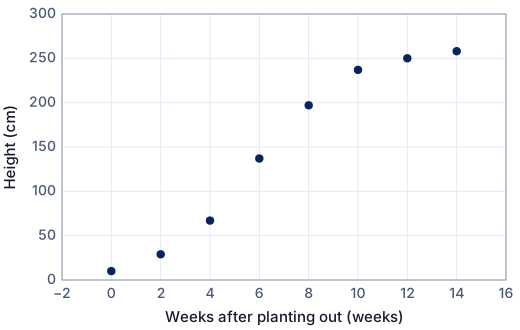
Scatter graph of height against weeks after planting out for the example data — Step 1 of any modelling IA: plot the data and describe the shape before fitting anything.

The method: estimate L, linearise, refine

The seed packet suggests a maximum height of about 270 cm, so start with L = 270. Linearise to find C and k, then refine L, C and k together by least squares.

Step 1 · Estimate the carrying capacity L

From the context, the values level off at about L = 270.

Step 2 · Linearise

Rearranging y = L/(1 + Ce^−kx) gives L/y − 1 = Ce^−kx, so ln(L/y − 1) = −kx + ln C: a straight line with gradient −k and intercept ln C.

Step 3 · Tabulate the sums

Sums for the least-squares line
i	x	ln(L/y − 1)	x²	x(ln(L/y − 1))	(ln(L/y − 1))²
1	0	3.2581	0	0.0000	10.615
2	2	2.1175	4	4.2350	4.4838
3	4	1.1085	16	4.4341	1.2288
4	6	−0.029632	36	−0.17779	0.00087804
5	8	−0.99274	64	−7.9420	0.98554
6	10	−1.9716	100	−19.716	3.8870
7	12	−2.5257	144	−30.309	6.3793
8	14	−3.0681	196	−42.953	9.4129
Σ	56.0000	−2.10360	560.000	−92.4277	36.9935

n = 8 points. The transformed values are rounded here; keep them unrounded in your calculator or spreadsheet.

Step 4 · Gradient

m = (nΣXY − ΣX ΣY) / (nΣX² − (ΣX)²)

m = (8 × (−92.4277) − 56.0000 × (−2.10360)) / (8 × 560.000 − 56.0000²) = −621.620 / 1344 = −0.4625

Here X = x and Y = ln(L/y − 1).

Step 5 · Intercept

X̄ = ΣX/n = 7.0000, Ȳ = ΣY/n = −0.26295

c = Ȳ − m X̄ = −0.26295 − (−0.4625) × 7.0000 = 2.975

The line of best fit always passes through the mean point (X̄, Ȳ).

Step 6 · Correlation

r = (nΣXY − ΣX ΣY) / √[(nΣX² − (ΣX)²)(nΣY² − (ΣY)²)] = −621.620 / √(1344 × 291.523) = −0.9931

r² = 0.9862: a very strong negative linear correlation between x and ln(L/y − 1).

Step 7 · First model

k = −(gradient) = 0.4625; C = e^2.975 = 19.58.

y = 270/(1 + 19.58e^−0.4625x)

Step 8 · How well does the first model fit?

For each point, the residual is the observed value minus the model's value: e = y − ŷ.

Residuals
i	x	y (data)	ŷ (model)	y − ŷ	(y − ŷ)²
1	0	10	13.12	−3.12	9.72
2	2	29	30.80	−1.80	3.26
3	4	67	66.19	0.807	0.651
4	6	137	121.6	15.4	238
5	8	197	181.9	15.1	227
6	10	237	226.5	10.5	110
7	12	250	250.9	−0.903	0.815
8	14	258	262.1	−4.09	16.7
Σ					606.1

Sum of squared residuals: SSR = Σ(y − ŷ)² = 606.1
Total sum of squares about the mean ȳ = 148.1: SST = Σ(y − ȳ)² = 72710
Coefficient of determination: R² = 1 − SSR/SST = 1 − 606.1/72710 = 0.9917
Root-mean-square error: RMSE = √(SSR/n) = 8.70 — a typical size of a residual, in the units of y.

Step 9 · Refine all three parameters

The estimate of L was a guess, so now minimise SSR over L, C and k together (iteratively, starting from the first model — this is what GDC logistic regression and Desmos do):

y = 260.1/(1 + 24.86e^−0.5482x)

The curve levels off at L = 260.1. It grows fastest at the point of inflection, where y = L/2 = 130.1 and x = ln C/k = 5.861.

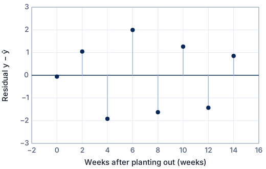
Step 10 · Residuals of the refined model

For each point, the residual is the observed value minus the model's value: e = y − ŷ.

Residuals
i	x	y (data)	ŷ (model)	y − ŷ	(y − ŷ)²
1	0	10	10.06	−0.0576	0.00332
2	2	29	27.95	1.05	1.09
3	4	67	68.92	−1.92	3.68
4	6	137	135.0	2.00	3.99
5	8	197	198.6	−1.63	2.65
6	10	237	235.7	1.26	1.59
7	12	250	251.4	−1.43	2.04
8	14	258	257.1	0.852	0.726
Σ					15.77

Sum of squared residuals: SSR = Σ(y − ŷ)² = 15.77
Total sum of squares about the mean ȳ = 148.1: SST = Σ(y − ȳ)² = 72710
Coefficient of determination: R² = 1 − SSR/SST = 1 − 15.77/72710 = 0.9998
Root-mean-square error: RMSE = √(SSR/n) = 1.40 — a typical size of a residual, in the units of y.

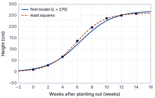
Graph of the data with the fitted logistic (first model (L = 270)) — Estimate L, linearise, refine: the fitted curves over the example data.

Residual plot for the logistic fitted to the example data — Residuals against x. Look for a pattern: random scatter about 0 means the model has captured the shape; a curve or a trend means it has not.

What the model tells you

L ≈ 260 cm: the height the plant levels off at, a little below the packet's 270 cm.
k ≈ 0.55 per week: the growth-rate constant. Early on, height grows by a factor of about e^k ≈ 1.7 each week.
The point of inflection, where growth is fastest, is at about 5.9 weeks and 130 cm — check this against the steepest part of the data.

The same on a GDC

Enter and plot the data first, then fit. The key sequences are for current operating systems; menus differ slightly between versions.

TI-84 Plus CE

Data: [stat] → 1: Edit… Type the x values in L1 and the y values in L2. To plot: [2nd] [y=] (STAT PLOT) → Plot1: On, Type: scatter, Xlist: L1, Ylist: L2, then [zoom] → 9: ZoomStat.
[stat] → CALC → B: Logistic, Xlist L1, Ylist L2, Store RegEQ Y1. Result y = c/(1 + a·e^(−bx)): the TI's c is L, a is C, b is k.

TI-Nspire CX

Data: Add a Lists & Spreadsheet page; name column A xs and column B ys and type the data. Add a Data & Statistics page (or a Graphs page with menu → Graph Entry/Edit → Scatter Plot) and choose xs and ys.
Statistics → Stat Calculations → Logistic (d = 0): y = c/(1 + a·e^(−bx)). Same letters as the TI.

Casio fx-CG50

Data: [MENU] → Statistics. Type the x values in List 1 and the y values in List 2. To plot: [F1] (GRAPH) → [F6] (SET): Graph Type Scatter, XList List1, YList List2; [EXIT], then [F1] (GRAPH1).
Statistics → [F2] (CALC) → [F3] (REG) → [F6] (▷) → [F5] (Lgst): y = c/(1 + a·e^(−bx)).

In Desmos

Free at desmos.com/calculator. In a regression, ~ means “fit this model”; subscripts are typed with an underscore (x_1 shows as x₁).

Data in x₁, y₁.
y_1 ~ L/(1 + C e^(-k x_1)).
If Desmos struggles, give it a hint by fixing L from the context first: y_1 ~ 270/(1 + C e^(-k x_1)), then free it.

More on technology in the IA: using Desmos, GeoGebra and Excel.

How to write it up in your IA

Explain why growth must level off in this context and where the estimate of L comes from.
Show the rearrangement to ln(L/y − 1) = −kx + ln C and the transformed table.
Show how C and k come from the line, then describe the refinement and report all three parameters.
Interpret L, k and the point of inflection in context.
Compare with an exponential model on the early data: where does it fail, and why?

These are the points to cover, not sentences to copy. Write every explanation in your own words, about your own data.

Common mistakes

Choosing L smaller than a data value (ln of a negative number).
Fitting a logistic to data that have not started to level off — L is then a guess, so say so.
Mixing the calculator's letters (c/(1 + a e^(−bx))) with your own.

Is this good enough for Criterion E?

The need for a ceiling is justified from the context.
The linearisation is derived and shown with a table.
L, C and k are found, refined, and interpreted in context (including the inflection point).
The model is compared with a simpler one (exponential or linear) using SSR or residuals.
HL: the logistic model is linked to the differential equation dy/dx = ky(1 − y/L), or the sensitivity to the estimate of L is analysed.

SL or HL? Criterion E asks for mathematics that fits your course. At SL, fitting with technology is fine when you explain the method and justify every choice. At HL, show more of the mathematics yourself — the last item in the list is an example. See Criterion E and Criterion D.

Frequently asked questions

How do I estimate L for a logistic model?

From the context if you can (a capacity, a population size, 100%), otherwise a little above the largest value once the data are clearly levelling off. Then let the regression refine it and report both.

Free: the IA checklist an examiner uses

Every check for Criteria A–E in a 4-page PDF, the mistakes that cost the most marks and a self-assessment grid. We'll email it with a short IA tip every few days, timed to your deadline if you give it. Free — no account, no payment.

Get the free checklist