IA modelling, step by step · Piecewise
Piecewise model, step by step: when the rule changes part-way
Some data follow one rule and then another: water heats steadily and then boils, a tariff changes at a threshold, a runner speeds up for the finish. Split the domain where the context says the rule changes, fit each piece, and join them.
Example data, invented for this guide. The context is realistic, but the numbers were made up to show the method. Use your own measured or sourced data in your IA.
When to use it
The shape of the data
- A sudden change of gradient (a kink) or a change of shape part-way through.
- One model fits the first part well but clearly fails on the rest.
The context
- A physical change of state (heating then boiling, melting).
- Rules with thresholds: tax bands, tariffs, speed limits.
- A process with phases: acceleration then steady speed.
Course fit: AI HL (piecewise models); domain notation is used everywhere. Justifying the split from the context is what makes it strong at any level.
The example data
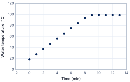
A pan of water is heated on a hob at a constant setting; a thermometer is read every minute until it has been boiling for a few minutes.
| i | x: Time (min) | y: Water temperature (°C) |
|---|---|---|
| 1 | 0 | 18.4 |
| 2 | 1 | 27.6 |
| 3 | 2 | 37.3 |
| 4 | 3 | 46.5 |
| 5 | 4 | 56.2 |
| 6 | 5 | 65.3 |
| 7 | 6 | 75 |
| 8 | 7 | 84.1 |
| 9 | 8 | 93.8 |
| 10 | 9 | 98.9 |
| 11 | 10 | 99.2 |
| 12 | 11 | 99 |
| 13 | 12 | 99.1 |
| 14 | 13 | 98.9 |
The method: split, fit each piece, join
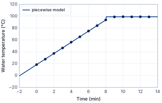
The water heats at a steady rate until it boils, then stays at boiling point. Split after x = 8 (the last reading before the temperature stops rising), fit a line to the first piece and a constant to the second, then find where they meet.
Step 1 · Split the domain
Split the data where the behaviour changes (from the graph and the context): piece 1 for x ≤ 8 (9 points), piece 2 for x > 8 (5 points).
Step 2 · Tabulate the sums for piece 1
| i | x | y | x² | xy | y² |
|---|---|---|---|---|---|
| 1 | 0 | 18.4 | 0 | 0 | 338.56 |
| 2 | 1 | 27.6 | 1 | 27.6 | 761.76 |
| 3 | 2 | 37.3 | 4 | 74.6 | 1391.29 |
| 4 | 3 | 46.5 | 9 | 139.5 | 2162.25 |
| 5 | 4 | 56.2 | 16 | 224.8 | 3158.44 |
| 6 | 5 | 65.3 | 25 | 326.5 | 4264.09 |
| 7 | 6 | 75 | 36 | 450 | 5625 |
| 8 | 7 | 84.1 | 49 | 588.7 | 7072.81 |
| 9 | 8 | 93.8 | 64 | 750.4 | 8798.44 |
| Σ | 36 | 504.2 | 204 | 2582.1 | 33572.64 |
n = 9 points.
Step 3 · Gradient
m = (nΣXY − ΣX ΣY) / (nΣX² − (ΣX)²)
m = (9 × 2582.1 − 36 × 504.2) / (9 × 204 − 36²) = 5087.7 / 540 = 9.422
Here X = x and Y = y.
Step 4 · Intercept
X̄ = ΣX/n = 4.0000, Ȳ = ΣY/n = 56.022
c = Ȳ − m X̄ = 56.022 − 9.422 × 4.0000 = 18.34
The line of best fit always passes through the mean point (X̄, Ȳ).
Step 5 · Correlation
r = (nΣXY − ΣX ΣY) / √[(nΣX² − (ΣX)²)(nΣY² − (ΣY)²)] = 5087.7 / √(540 × 47936.12) = 1.000
r² = 1.000: a very strong positive linear correlation between x and y.
Step 6 · Piece 2: a constant
The context says the second piece should be level, so the least-squares constant is the mean of its y values: y = 99.02.
Step 7 · Where the pieces meet
Set the two pieces equal: 9.422x + 18.34 = 99.02, so x = 8.564, y = 99.02. Using this as the boundary makes the model continuous (no jump), which usually matches the context better than the split you started with.
Model: y = 9.422x + 18.34 for x ≤ 8; y = 99.02 for x > 8
Step 8 · Residuals and goodness of fit
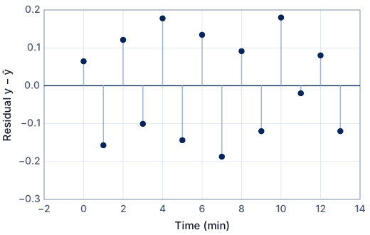
For each point, the residual is the observed value minus the model's value: e = y − ŷ.
| i | x | y (data) | ŷ (model) | y − ŷ | (y − ŷ)² |
|---|---|---|---|---|---|
| 1 | 0 | 18.4 | 18.34 | 0.0644 | 0.00415 |
| 2 | 1 | 27.6 | 27.76 | −0.157 | 0.0247 |
| 3 | 2 | 37.3 | 37.18 | 0.121 | 0.0147 |
| 4 | 3 | 46.5 | 46.60 | −0.101 | 0.0101 |
| 5 | 4 | 56.2 | 56.02 | 0.178 | 0.0316 |
| 6 | 5 | 65.3 | 65.44 | −0.144 | 0.0207 |
| 7 | 6 | 75 | 74.87 | 0.134 | 0.0181 |
| 8 | 7 | 84.1 | 84.29 | −0.187 | 0.0351 |
| 9 | 8 | 93.8 | 93.71 | 0.0911 | 0.00830 |
| 10 | 9 | 98.9 | 99.02 | −0.120 | 0.0144 |
| 11 | 10 | 99.2 | 99.02 | 0.180 | 0.0324 |
| 12 | 11 | 99 | 99.02 | −0.0200 | 0.000400 |
| 13 | 12 | 99.1 | 99.02 | 0.0800 | 0.00640 |
| 14 | 13 | 98.9 | 99.02 | −0.120 | 0.0144 |
| Σ | 0.2354 |
- Sum of squared residuals: SSR = Σ(y − ŷ)² = 0.2354
- Total sum of squares about the mean ȳ = 71.38: SST = Σ(y − ȳ)² = 11270
- Coefficient of determination: R² = 1 − SSR/SST = 1 − 0.2354/11270 = 1.000
- Root-mean-square error: RMSE = √(SSR/n) = 0.130 — a typical size of a residual, in the units of y.
What the model tells you
- Gradient of piece 1 ≈ 9.42 °C per minute: the heating rate at this hob setting.
- Piece 2 ≈ 99.0 °C: the boiling point. It is slightly below 100 °C, which could be thermometer calibration or air pressure — good reflection.
- The pieces meet at about 8.6 minutes: the model's estimate of when boiling starts.
The same on a GDC
Enter and plot the data first, then fit. The key sequences are for current operating systems; menus differ slightly between versions.
TI-84 Plus CE
- Data: [stat] → 1: Edit… Type the x values in L1 and the y values in L2. To plot: [2nd] [y=] (STAT PLOT) → Plot1: On, Type: scatter, Xlist: L1, Ylist: L2, then [zoom] → 9: ZoomStat.
- Put the first piece (x ≤ 8) in L1, L2 and the second in L3, L4.
- LinReg(ax+b) L1, L2 for piece 1; for a constant piece, 1-Var Stats L4 gives the mean.
- Graph each piece with a domain: Y1 = (9.422X + 18.34)/(X ≤ 8.564) draws only where the condition is true.
TI-Nspire CX
- Data: Add a Lists & Spreadsheet page; name column A xs and column B ys and type the data. Add a Data & Statistics page (or a Graphs page with menu → Graph Entry/Edit → Scatter Plot) and choose xs and ys.
- Fit each piece's columns with Linear Regression; define the model with a template: menu → Functions… or type a piecewise function with the { template.
Casio fx-CG50
- Data: [MENU] → Statistics. Type the x values in List 1 and the y values in List 2. To plot: [F1] (GRAPH) → [F6] (SET): Graph Type Scatter, XList List1, YList List2; [EXIT], then [F1] (GRAPH1).
- Fit each piece's lists separately with REG; in Graph mode add a domain after a comma: Y1 = 9.422X + 18.34, [0, 8.564].
In Desmos
Free at desmos.com/calculator. In a regression, ~ means “fit this model”; subscripts are typed with an underscore (x_1 shows as x₁).
- Two tables (one per piece), each with its own regression:
y_1 ~ m x_1 + candy_2 ~ k. - Draw with domains:
y = 9.422x + 18.34 {0 ≤ x ≤ 8.564}andy = 99.02 {x ≥ 8.564}.
More on technology in the IA: using Desmos, GeoGebra and Excel.
How to write it up in your IA
- Explain from the context why the rule changes and where.
- Fit each piece and show its working; justify the form of each piece.
- Find where the pieces meet and discuss whether the model should be continuous.
- Write the model with its domains in correct notation.
- Discuss how sensitive the result is to where you split (try moving the split by one point).
These are the points to cover, not sentences to copy. Write every explanation in your own words, about your own data.
Common mistakes
- Splitting where it makes the numbers look best rather than where the context says.
- Pieces that do not meet when the context has no jump.
- Missing or overlapping domains in the written model.
Is this good enough for Criterion E?
- The split is justified by the context and visible in the data.
- Each piece is fitted and justified; the join is found algebraically.
- The model is written with correct domain notation.
- Sensitivity to the split point is tested.
- HL: the split point is estimated by minimising the total SSR over possible splits.
SL or HL? Criterion E asks for mathematics that fits your course. At SL, fitting with technology is fine when you explain the method and justify every choice. At HL, show more of the mathematics yourself — the last item in the list is an example. See Criterion E and Criterion D.
Frequently asked questions
Where should I split the data for a piecewise model?
Where the context says the rule changes (boiling, a tariff threshold), confirmed by the graph. Then check how much the parameters change if you move the split by one point.
Free: the IA checklist an examiner uses
Every check for Criteria A–E in a 4-page PDF, the mistakes that cost the most marks and a self-assessment grid. We'll email it with a short IA tip every few days, timed to your deadline if you give it. Free — no account, no payment.
While you wait for the email: read the full modelling workflow →