IA modelling, step by step · Logarithmic

Logarithmic model, step by step: y = a ln x + b

AA SLAA HLAI HL

When something keeps growing but more and more slowly — skills, learning, diminishing returns — try y = a ln x + b. Plot y against ln x: if the points lie on a line, its gradient is a and its intercept is b.

Guidance based on the checklist Pete Bromfield — an IB examiner and former Head of Maths — uses with his own students. Not affiliated with or endorsed by the IB.

Example data, invented for this guide. The context is realistic, but the numbers were made up to show the method. Use your own measured or sourced data in your IA.

When to use it

The shape of the data

Steep at first, then flattening out, but with no sign of a ceiling.
Equal ratios of x give equal steps in y (doubling x adds the same amount each time).
A plot of y against ln x is close to straight.

The context

Learning and practice: speed or score against time spent.
Diminishing returns: sales against advertising spend, yield against fertiliser.
Scales that are already logarithmic: decibels, pH, earthquake magnitude.

Course fit: AA (logarithms and the laws of logs) and AI HL (logarithmic models and linearising data). At AI SL it is fine in an IA if you explain the method as new to you.

The example data

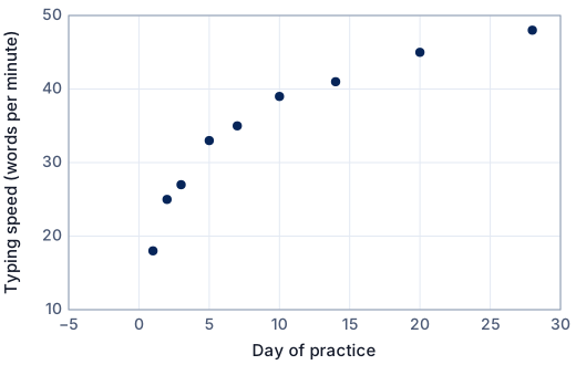
A student learning to touch-type records their speed on a 1-minute test at the end of chosen practice days.

Example data: typing speed and day of practice
i	x: Day of practice	y: Typing speed (words per minute)
1	1	18
2	2	25
3	3	27
4	5	33
5	7	35
6	10	39
7	14	41
8	20	45
9	28	48

Scatter graph of typing speed against day of practice for the example data — Step 1 of any modelling IA: plot the data and describe the shape before fitting anything.

The method: linearise, fit a line, back-substitute

Transform x to X = ln x, fit the least-squares line to (ln x, y) with the usual sums, then read a and b from its gradient and intercept.

Step 1 · Linearise

If y = a ln x + b, then plotting y against X = ln x gives a straight line with gradient a and intercept b. Transform the x values (natural log, ln):

Step 2 · Tabulate the sums

Sums for the least-squares line
i	ln x	y	(ln x)²	(ln x)y	y²
1	0	18	0	0	324
2	0.69315	25	0.48045	17.329	625
3	1.0986	27	1.2069	29.663	729
4	1.6094	33	2.5903	53.111	1089
5	1.9459	35	3.7866	68.107	1225
6	2.3026	39	5.3019	89.801	1521
7	2.6391	41	6.9646	108.20	1681
8	2.9957	45	8.9744	134.81	2025
9	3.3322	48	11.104	159.95	2304
Σ	16.6167	311.000	40.4088	660.965	11523.0

n = 9 points. The transformed values are rounded here; keep them unrounded in your calculator or spreadsheet.

Step 3 · Gradient

m = (nΣXY − ΣX ΣY) / (nΣX² − (ΣX)²)

m = (9 × 660.965 − 16.6167 × 311.000) / (9 × 40.4088 − 16.6167²) = 780.900 / 87.5647 = 8.918

Here X = ln x and Y = y.

Step 4 · Intercept

X̄ = ΣX/n = 1.8463, Ȳ = ΣY/n = 34.556

c = Ȳ − m X̄ = 34.556 − 8.918 × 1.8463 = 18.09

The line of best fit always passes through the mean point (X̄, Ȳ).

Step 5 · Correlation

r = (nΣXY − ΣX ΣY) / √[(nΣX² − (ΣX)²)(nΣY² − (ΣY)²)] = 780.900 / √(87.5647 × 6986) = 0.9984

r² = 0.9969: a very strong positive linear correlation between ln x and y.

Step 6 · Back-substitute

Gradient a = 8.918 and intercept b = 18.09, so

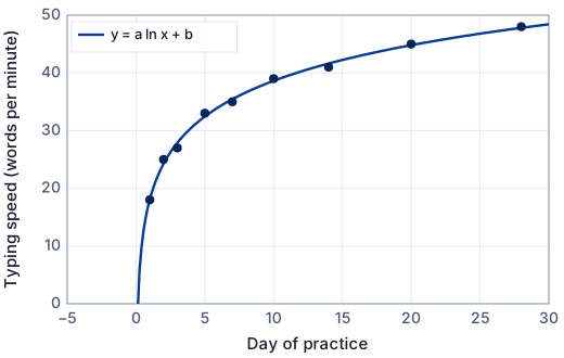
y = 8.918 ln x + 18.09

The model grows without limit but ever more slowly: each time x is multiplied by e (≈ 2.718), y goes up by a; each doubling of x adds a ln 2 = 6.181.

Step 7 · Residuals and goodness of fit

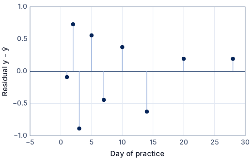
For each point, the residual is the observed value minus the model's value: e = y − ŷ.

Residuals
i	x	y (data)	ŷ (model)	y − ŷ	(y − ŷ)²
1	1	18	18.09	−0.0903	0.00816
2	2	25	24.27	0.728	0.530
3	3	27	27.89	−0.888	0.788
4	5	33	32.44	0.557	0.310
5	7	35	35.44	−0.444	0.197
6	10	39	38.62	0.375	0.141
7	14	41	41.63	−0.625	0.391
8	20	45	44.81	0.194	0.0376
9	28	48	47.81	0.193	0.0373
Σ					2.440

Sum of squared residuals: SSR = Σ(y − ŷ)² = 2.440
Total sum of squares about the mean ȳ = 34.56: SST = Σ(y − ȳ)² = 776.2
Coefficient of determination: R² = 1 − SSR/SST = 1 − 2.440/776.2 = 0.9969
Root-mean-square error: RMSE = √(SSR/n) = 0.521 — a typical size of a residual, in the units of y.

Because y itself was not transformed, this is the same as least squares on the original data, and R² = r² of the (ln x, y) line.

Graph of the data with the fitted logarithmic (y = a ln x + b) — Linearise, fit a line, back-substitute: the fitted curve over the example data.

Residual plot for the logarithmic fitted to the example data — Residuals against x. Look for a pattern: random scatter about 0 means the model has captured the shape; a curve or a trend means it has not.

What the model tells you

a ≈ 8.92: each time the number of practice days is multiplied by e, speed goes up by about 8.9 wpm; each doubling of practice adds about 6.2 wpm.
b ≈ 18.1: the model's speed on day 1 (ln 1 = 0). Here that is inside the data, so it is meaningful.
The model never levels off: it predicts 51.0 wpm on day 40 and keeps rising for ever, which is unrealistic for typing speed. Say this, and state the domain 1 ≤ x ≤ 28 days.

The same on a GDC

Enter and plot the data first, then fit. The key sequences are for current operating systems; menus differ slightly between versions.

TI-84 Plus CE

Data: [stat] → 1: Edit… Type the x values in L1 and the y values in L2. To plot: [2nd] [y=] (STAT PLOT) → Plot1: On, Type: scatter, Xlist: L1, Ylist: L2, then [zoom] → 9: ZoomStat.
[stat] → CALC → 9: LnReg, Xlist L1, Ylist L2, Store RegEQ Y1.
Careful: the TI writes y = a + b ln x, so its a is our b and its b is our a.
To see the linearisation: set L3 = ln(L1) (type it in L3's header) and run LinReg(ax+b) with L3, L2 — you get the same numbers.

TI-Nspire CX

Data: Add a Lists & Spreadsheet page; name column A xs and column B ys and type the data. Add a Data & Statistics page (or a Graphs page with menu → Graph Entry/Edit → Scatter Plot) and choose xs and ys.
menu → Statistics → Stat Calculations → Logarithmic Regression, X List xs, Y List ys. Result y = a + b·ln(x).
Or add a column lnx := ln(xs) and use Linear Regression on lnx and ys.

Casio fx-CG50

Data: [MENU] → Statistics. Type the x values in List 1 and the y values in List 2. To plot: [F1] (GRAPH) → [F6] (SET): Graph Type Scatter, XList List1, YList List2; [EXIT], then [F1] (GRAPH1).
Statistics → [F2] (CALC) → [F3] (REG) → [F6] (▷) → [F1] (Log). Result y = a + b·ln x.
Or fill List 3 with ln List 1 (type it in List 3's header) and do [F1] (X) linear regression with XList List3.

In Desmos

Free at desmos.com/calculator. In a regression, ~ means “fit this model”; subscripts are typed with an underscore (x_1 shows as x₁).

Data in x₁, y₁.
Type y_1 ~ a ln(x_1) + b. Because this model is linear in a and b, Desmos's answer is exactly the least-squares line in (ln x, y).
Add a column ln(x_1) to the table and plot it against y₁ to show the linearised data.

More on technology in the IA: using Desmos, GeoGebra and Excel.

How to write it up in your IA

Explain why the growth-slowing shape and the context suggest a logarithm.
Show the transformed table (ln x) and the straight-line plot: this is the justification for the model.
Show the least-squares calculation once, then how a and b come from the gradient and intercept.
Interpret a in context (the gain per doubling is a vivid way to put it).
Discuss the domain: ln x needs x > 0, and the model grows without limit.
Compare with at least one other model (linear, power or logistic) using SSR or a residual plot.

These are the points to cover, not sentences to copy. Write every explanation in your own words, about your own data.

Common mistakes

Using log₁₀ in one place and ln in another: the value of a changes. Pick one and say which.
Swapping a and b because the calculator's form is y = a + b ln x.
Including x = 0 (ln 0 is undefined): shift x so it starts at 1 and say so.
Judging the model by r of the transformed data only, without looking at the fit to the original data.

Is this good enough for Criterion E?

The logarithmic shape is justified from the graph and the context.
The linearisation is shown (table and a plot of y against ln x).
a and b are found from the line and back-substituted correctly.
The model is interpreted in context and its domain and long-term behaviour are discussed.
It is compared with another model on the same data.
HL: the logarithm laws are used to justify the transformation, or the model is compared with a bounded (logistic) one.

SL or HL? Criterion E asks for mathematics that fits your course. At SL, fitting with technology is fine when you explain the method and justify every choice. At HL, show more of the mathematics yourself — the last item in the list is an example. See Criterion E and Criterion D.

Frequently asked questions

Can I use log base 10 instead of ln?

Yes: y = a log₁₀ x + b is the same family of curves with a different a (a₁₀ = a × ln 10). Use one base throughout and say which.

Free: the IA checklist an examiner uses

Every check for Criteria A–E in a 4-page PDF, the mistakes that cost the most marks and a self-assessment grid. We'll email it with a short IA tip every few days, timed to your deadline if you give it. Free — no account, no payment.

Get the free checklist