IA modelling, step by step · Cubic and polynomials

Cubic and polynomial models — and why a perfect fit can be the worst model

AA SLAA HLAI SLAI HL

Adding terms to a polynomial always lowers the sum of squared residuals on the data you fitted — until a curve of degree n − 1 passes through every point. This page fits four polynomials to the same data and shows why the ‘perfect’ one is useless.

Guidance based on the checklist Pete Bromfield — an IB examiner and former Head of Maths — uses with his own students. Not affiliated with or endorsed by the IB.

Example data, invented for this guide. The context is realistic, but the numbers were made up to show the method. Use your own measured or sourced data in your IA.

When to use it

The shape of the data

A cubic: one rise and one fall with an asymmetric shape, or a point of inflection.
More turning points than a quadratic can have — but ask whether the context really has them.

The context

Volume-type relationships (a box, a container) where x³ appears naturally.
An asymmetric rise and fall where a quadratic is clearly too symmetric.
Never just because a higher degree gives a higher R².

Course fit: Cubic models are AI SL; polynomial functions are AA (especially HL). Discussing overfitting is excellent reflection at any level.

The example data

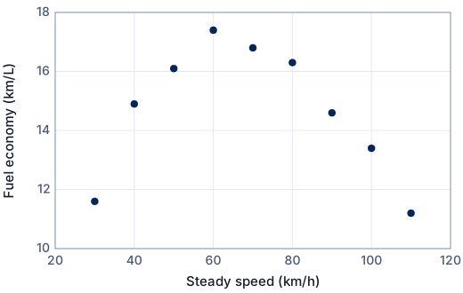
A family car's trip computer shows fuel economy after driving at each steady speed on a flat road for 5 minutes.

Example data: fuel economy and steady speed
i	x: Steady speed (km/h)	y: Fuel economy (km/L)
1	30	11.6
2	40	14.9
3	50	16.1
4	60	17.4
5	70	16.8
6	80	16.3
7	90	14.6
8	100	13.4
9	110	11.2

Scatter graph of fuel economy against steady speed for the example data — Step 1 of any modelling IA: plot the data and describe the shape before fitting anything.

Degree 1: a straight line

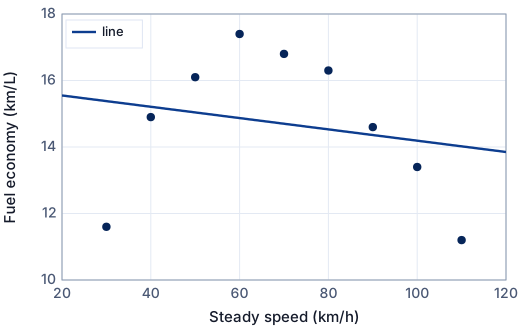
The data clearly rise and fall, so a line should fail. It is still worth fitting: it is the baseline every other model must beat.

Step 2 · Gradient

m = (nΣXY − ΣX ΣY) / (nΣX² − (ΣX)²)

m = (9 × 9159 − 630 × 132.3) / (9 × 50100 − 630²) = −918 / 54000 = −0.01700

Here X = x and Y = y.

Step 3 · Intercept

X̄ = ΣX/n = 70.000, Ȳ = ΣY/n = 14.700

c = Ȳ − m X̄ = 14.700 − (−0.01700) × 70.000 = 15.89

The line of best fit always passes through the mean point (X̄, Ȳ).

Step 4 · Correlation

r = (nΣXY − ΣX ΣY) / √[(nΣX² − (ΣX)²)(nΣY² − (ΣY)²)] = −918 / √(54000 × 358.38) = −0.2087

r² = 0.04355: very little or no negative linear correlation between x and y.

Step 5 · The model

y = −0.01700x + 15.89

The gradient −0.01700 is the change in y for each 1 unit increase in x; the intercept 15.89 is the model's value of y at x = 0 — say whether that means anything in your context.

Step 6 · Residuals and goodness of fit

For each point, the residual is the observed value minus the model's value: e = y − ŷ.

Residuals
i	x	y (data)	ŷ (model)	y − ŷ	(y − ŷ)²
1	30	11.6	15.38	−3.78	14.3
2	40	14.9	15.21	−0.310	0.0961
3	50	16.1	15.04	1.06	1.12
4	60	17.4	14.87	2.53	6.40
5	70	16.8	14.70	2.10	4.41
6	80	16.3	14.53	1.77	3.13
7	90	14.6	14.36	0.240	0.0576
8	100	13.4	14.19	−0.790	0.624
9	110	11.2	14.02	−2.82	7.95
Σ					38.09

Sum of squared residuals: SSR = Σ(y − ŷ)² = 38.09
Total sum of squares about the mean ȳ = 14.70: SST = Σ(y − ȳ)² = 39.82
Coefficient of determination: R² = 1 − SSR/SST = 1 − 38.09/39.82 = 0.04355
Root-mean-square error: RMSE = √(SSR/n) = 2.06 — a typical size of a residual, in the units of y.

For a least-squares line, R² equals r² (0.04355).

Graph of the data with the fitted straight line (least squares) (line) — A straight line: the fitted curve over the example data.

Degree 2: a quadratic

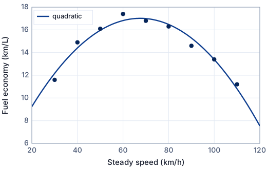
One turning point, as the context suggests (there is a most economical speed).

Step 2 · The normal equations

Least squares chooses a, b, c to make SSR = Σ(y − ax² − bx − c)² as small as possible. Setting the partial derivatives of SSR to zero gives three linear equations:

399570000a + 4347000b + 50100c = 711590 (Σx⁴, Σx³, Σx², Σx²y)
4347000a + 50100b + 630c = 9159 (Σx³, Σx², Σx, Σxy)
50100a + 630b + 9c = 132.3 (Σx², Σx, n, Σy)

HL students can derive these by differentiating SSR with respect to each parameter; at SL it is enough to say the calculator minimises SSR.

Step 3 · Solve (matrix or GDC)

Solving the 3 × 3 system (with a matrix inverse, the simultaneous-equation solver, or directly with quadratic regression):

a = −0.003442, b = 0.4648, c = 1.321

y = −0.003442x² + 0.4648x + 1.321

Turning point: x = −b/(2a) = 67.53, y = 17.02.

Step 4 · Residuals and goodness of fit

For each point, the residual is the observed value minus the model's value: e = y − ŷ.

Residuals
i	x	y (data)	ŷ (model)	y − ŷ	(y − ŷ)²
1	30	11.6	12.17	−0.568	0.322
2	40	14.9	14.41	0.493	0.243
3	50	16.1	15.96	0.142	0.0202
4	60	17.4	16.82	0.580	0.336
5	70	16.8	16.99	−0.194	0.0378
6	80	16.3	16.48	−0.180	0.0325
7	90	14.6	15.28	−0.678	0.459
8	100	13.4	13.39	0.0130	0.000170
9	110	11.2	10.81	0.392	0.154
Σ					1.605

Sum of squared residuals: SSR = Σ(y − ŷ)² = 1.605
Total sum of squares about the mean ȳ = 14.70: SST = Σ(y − ȳ)² = 39.82
Coefficient of determination: R² = 1 − SSR/SST = 1 − 1.605/39.82 = 0.9597
Root-mean-square error: RMSE = √(SSR/n) = 0.422 — a typical size of a residual, in the units of y.

For a quadratic, quote R² (not r, which measures linear correlation only).

Graph of the data with the fitted quadratic regression (quadratic) — A quadratic: the fitted curve over the example data.

Degree 3: a cubic

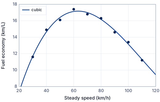
A cubic can be asymmetric — economy may fall off faster at high speed (air resistance grows with speed squared) than at low speed.

Step 1 · Fit by least squares (technology)

A degree-3 polynomial has 4 parameters. Least squares chooses them to minimise SSR; the normal equations are a 4 × 4 linear system, so in practice use a GDC (cubic regression), Desmos or a spreadsheet.

y = 0.00002887x³ − 0.009505x² + 0.8552x − 6.198

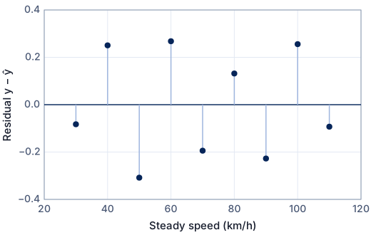
Step 2 · Residuals and goodness of fit

For each point, the residual is the observed value minus the model's value: e = y − ŷ.

Residuals
i	x	y (data)	ŷ (model)	y − ŷ	(y − ŷ)²
1	30	11.6	11.68	−0.0828	0.00686
2	40	14.9	14.65	0.251	0.0628
3	50	16.1	16.41	−0.308	0.0950
4	60	17.4	17.13	0.268	0.0718
5	70	16.8	16.99	−0.194	0.0378
6	80	16.3	16.17	0.132	0.0173
7	90	14.6	14.83	−0.227	0.0517
8	100	13.4	13.14	0.256	0.0653
9	110	11.2	11.29	−0.0929	0.00864
Σ					0.4171

Sum of squared residuals: SSR = Σ(y − ŷ)² = 0.4171
Total sum of squares about the mean ȳ = 14.70: SST = Σ(y − ȳ)² = 39.82
Coefficient of determination: R² = 1 − SSR/SST = 1 − 0.4171/39.82 = 0.9895
Root-mean-square error: RMSE = √(SSR/n) = 0.215 — a typical size of a residual, in the units of y.

Adding parameters never increases SSR, so a higher-degree polynomial always “fits better” on the data it was fitted to. Judge it on the context, the shape between and beyond the points, and on data it was not fitted to.

Graph of the data with the fitted cubic regression (cubic) — A cubic: the fitted curve over the example data.

Residual plot for the cubic regression fitted to the example data — Residuals against x. Look for a pattern: random scatter about 0 means the model has captured the shape; a curve or a trend means it has not.

Degree 8: a curve through every point

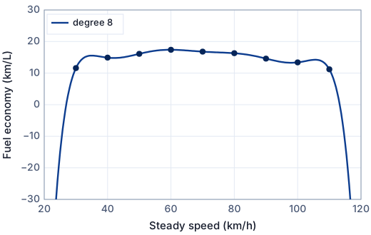
With nine points, a degree-8 polynomial passes exactly through all of them. SSR is 0 and R² is 1. Here is why that is a bad model.

Step 1 · Fit by least squares (technology)

A degree-8 polynomial has 9 parameters: with 9 points it passes through every one of them exactly. Its coefficients are not worth quoting — the point is what it does.

Step 2 · Residuals and goodness of fit

For each point, the residual is the observed value minus the model's value: e = y − ŷ.

Residuals
i	x	y (data)	ŷ (model)	y − ŷ	(y − ŷ)²
1	30	11.6	11.60	0.00	0.00
2	40	14.9	14.90	0.00	0.00
3	50	16.1	16.10	0.00	0.00
4	60	17.4	17.40	0.00	0.00
5	70	16.8	16.80	0.00	0.00
6	80	16.3	16.30	0.00	0.00
7	90	14.6	14.60	0.00	0.00
8	100	13.4	13.40	0.00	0.00
9	110	11.2	11.20	0.00	0.00
Σ					0.000

Sum of squared residuals: SSR = Σ(y − ŷ)² = 0.000
Total sum of squares about the mean ȳ = 14.70: SST = Σ(y − ȳ)² = 39.82
Coefficient of determination: R² = 1 − SSR/SST = 1 − 0.000/39.82 = 1.000
Root-mean-square error: RMSE = √(SSR/n) = 0.00 — a typical size of a residual, in the units of y.

Graph of the data with the fitted polynomial (degree 8) — A curve through every point: the fitted curve over the example data.

Comparing the methods

The same data, different methods
Method	Parameters	SSR	R²	RMSE
a straight line	2	38.09	0.04355	2.06
a quadratic	3	1.605	0.9597	0.422
a cubic	4	0.4171	0.9895	0.215
a curve through every point	9	0.000	1.000	0.00

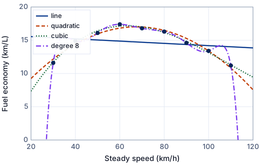
All the fitted models drawn over the example data on one graph — The models side by side. Where do they differ most — between the points, or beyond them?

Least squares gives the smallest SSR of any curve of its type, because that is what it minimises. A model through chosen points depends on which points you choose; test that by choosing others. For a fair comparison between different types, also compare the number of parameters and the shape beyond the data — see choosing and comparing models.

What the model tells you

SSR falls every time the degree goes up: that is guaranteed, because each polynomial includes the previous one as a special case.
The degree-8 curve predicts −15.1 km/L at 25 km/h and −12.3 km/L at 115 km/h: negative fuel economy. It is fitting the measurement noise, not the car. This is overfitting.
The cubic is a real improvement on the quadratic (its SSR is 0.26 times the quadratic's) for one extra parameter, and its asymmetry has a physical reason. That is a defensible choice; degree 8 is not.

The same on a GDC

Enter and plot the data first, then fit. The key sequences are for current operating systems; menus differ slightly between versions.

TI-84 Plus CE

Data: [stat] → 1: Edit… Type the x values in L1 and the y values in L2. To plot: [2nd] [y=] (STAT PLOT) → Plot1: On, Type: scatter, Xlist: L1, Ylist: L2, then [zoom] → 9: ZoomStat.
[stat] → CALC → 6: CubicReg (and 7: QuartReg for degree 4), Xlist L1, Ylist L2. Shows R².
There is no degree-8 regression on a GDC: use Desmos or a spreadsheet (LINEST) if you want to demonstrate overfitting.

TI-Nspire CX

Data: Add a Lists & Spreadsheet page; name column A xs and column B ys and type the data. Add a Data & Statistics page (or a Graphs page with menu → Graph Entry/Edit → Scatter Plot) and choose xs and ys.
Statistics → Stat Calculations → Cubic Regression (or Quartic Regression).

Casio fx-CG50

Data: [MENU] → Statistics. Type the x values in List 1 and the y values in List 2. To plot: [F1] (GRAPH) → [F6] (SET): Graph Type Scatter, XList List1, YList List2; [EXIT], then [F1] (GRAPH1).
Statistics → [F2] (CALC) → [F3] (REG) → [F4] (X³); [F5] (X⁴) for a quartic.

In Desmos

Free at desmos.com/calculator. In a regression, ~ means “fit this model”; subscripts are typed with an underscore (x_1 shows as x₁).

y_1 ~ a x_1^3 + b x_1^2 + c x_1 + d for a cubic.
Degree 8 (to show overfitting): y_1 ~ a x_1^8 + b x_1^7 + c x_1^6 + d x_1^5 + f x_1^4 + g x_1^3 + h x_1^2 + j x_1 + k; avoid the letter e, which Desmos reads as Euler's number.
Zoom out beyond the data to see what each polynomial predicts.

More on technology in the IA: using Desmos, GeoGebra and Excel.

How to write it up in your IA

Justify the degree from the context (how many turning points should there be?), not from R².
Show SSR and R² for each degree in one table, with the number of parameters.
Show what each model predicts between the points and just beyond the data, and whether that is sensible.
Choose the simplest model that captures the shape, and say why the extra parameters of a higher degree are not justified.
If you can, test the models on data you did not use to fit them (see the comparing page).

These are the points to cover, not sentences to copy. Write every explanation in your own words, about your own data.

Common mistakes

Choosing the model with the highest R² without looking at its shape.
Using a high-degree polynomial to extrapolate.
Quoting eight coefficients to 3 s.f.: rounding changes a high-degree polynomial dramatically.

Is this good enough for Criterion E?

The degree is justified by the context and the number of turning points.
Several degrees are compared with SSR/R² and the number of parameters.
Behaviour between and beyond the data is checked for each candidate.
Overfitting is recognised and discussed.
HL: an adjusted measure (for example, comparing on held-out points, or penalising extra parameters) is used to choose the degree.

SL or HL? Criterion E asks for mathematics that fits your course. At SL, fitting with technology is fine when you explain the method and justify every choice. At HL, show more of the mathematics yourself — the last item in the list is an example. See Criterion E and Criterion D.

Frequently asked questions

Is a higher R² always a better model?

No. For polynomials, R² can only go up as you add terms, even when the extra terms fit noise. Choose the simplest model whose shape makes sense in the context and that predicts well on data it was not fitted to.

Free: the IA checklist an examiner uses

Every check for Criteria A–E in a 4-page PDF, the mistakes that cost the most marks and a self-assessment grid. We'll email it with a short IA tip every few days, timed to your deadline if you give it. Free — no account, no payment.

Get the free checklist