IA modelling, step by step · Quadratic
Quadratic model, step by step: three points, completing the square and regression
Three ways to fit y = ax² + bx + c to the same data: solve three simultaneous equations through three points, build the vertex form y = a(x − h)² + k from the turning point, and use least-squares regression. Then compare all three with the sum of squared residuals.
Example data, invented for this guide. The context is realistic, but the numbers were made up to show the method. Use your own measured or sourced data in your IA.
When to use it
The shape of the data
- One turning point (a single peak or trough) and roughly symmetrical sides.
- The first differences of y change at a steady rate (constant second differences for equally spaced x).
The context
- Projectiles and anything thrown or sprayed (constant acceleration).
- Area, cost or profit that rises then falls (optimisation).
- Shapes with a symmetric curve: arches, bridges, the cross-section of a bowl or dish.
Course fit: Every course. Quadratics and completing the square are core AA; AI uses quadratic models with technology. Solving the 3 × 3 system with matrices is HL (AA or AI), but a GDC equation solver is fine at SL.
The example data
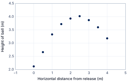
A basketball free throw is filmed side-on; the ball's centre is read from video frames against a scale on the wall.
| i | x: Horizontal distance from release (m) | y: Height of ball (m) |
|---|---|---|
| 1 | 0 | 2.12 |
| 2 | 0.5 | 2.66 |
| 3 | 1 | 3.33 |
| 4 | 1.5 | 3.72 |
| 5 | 2 | 3.93 |
| 6 | 2.5 | 4.02 |
| 7 | 3 | 3.87 |
| 8 | 3.5 | 3.6 |
| 9 | 4 | 3.18 |
Method 1: three points and simultaneous equations
A quadratic has three unknowns, so three points fix it exactly. Choose points spread across the data — the first, middle and last here — and solve the 3 × 3 system by elimination, then check it with matrices.
Step 1 · Substitute three points
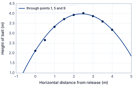
Using points 1, 5, 9 of the data, spread across the whole range: (0, 2.12), (2, 3.93), (4, 3.18). Each must satisfy y = ax² + bx + c:
- 0a + 0b + c = 2.12
- 4a + 2b + c = 3.93
- 16a + 4b + c = 3.18
Step 2 · Eliminate c
Subtract equation (1) from (2) and from (3):
- (2) − (1): 4a + 2b = 1.81
- (3) − (1): 16a + 4b = 1.06
Divide (4) by 2 and (5) by 4 (because x₂² − x₁² = (x₂ − x₁)(x₂ + x₁)):
- 2a + b = 0.905
- 4a + b = 0.265
Step 3 · Solve for a, then b, then c
(7) − (6): 2a = −0.64, so a = −0.3200.
From (6): b = 0.905 − 2 × (−0.3200) = 1.545.
From (1): c = 2.12 − 0 × (−0.3200) − 0 × 1.545 = 2.120.
Carry the unrounded values forward (store them in your calculator); rounded values give slightly different answers.
Step 4 · Check with matrices
The same system as a matrix equation AX = B:
| 0 | 0 | 1 |
| 4 | 2 | 1 |
| 16 | 4 | 1 |
| a |
| b |
| c |
| 2.12 |
| 3.93 |
| 3.18 |
X = A⁻¹B on a GDC (or the simultaneous-equation solver) gives the same a = −0.3200, b = 1.545, c = 2.120.
Step 5 · Complete the square to find the turning point
y = −0.3200(x² − 4.828x) + 2.120 (factor a out of the x terms: b/a = −4.828)
y = −0.3200[(x − 2.414)² − 5.828] + 2.120 (half of b/a is −2.414; subtract its square)
y = −0.3200(x − 2.414)² + 3.985
So the turning point is (h, k) = (2.414, 3.985): h = −b/(2a) and k = c − b²/(4a). Since a < 0 this is a maximum.
Step 6 · Residuals and goodness of fit
For each point, the residual is the observed value minus the model's value: e = y − ŷ.
| i | x | y (data) | ŷ (model) | y − ŷ | (y − ŷ)² |
|---|---|---|---|---|---|
| 1 | 0 | 2.12 | 2.120 | 0.00 | 0.00 |
| 2 | 0.5 | 2.66 | 2.813 | −0.152 | 0.0233 |
| 3 | 1 | 3.33 | 3.345 | −0.0150 | 0.000225 |
| 4 | 1.5 | 3.72 | 3.718 | 0.00250 | 0.00000625 |
| 5 | 2 | 3.93 | 3.930 | 0.00 | 0.00 |
| 6 | 2.5 | 4.02 | 3.982 | 0.0375 | 0.00141 |
| 7 | 3 | 3.87 | 3.875 | −0.00500 | 0.0000250 |
| 8 | 3.5 | 3.6 | 3.607 | −0.00750 | 0.0000562 |
| 9 | 4 | 3.18 | 3.180 | 0.00 | 0.00 |
| Σ | 0.02497 |
- Sum of squared residuals: SSR = Σ(y − ŷ)² = 0.02497
- Total sum of squares about the mean ȳ = 3.381: SST = Σ(y − ȳ)² = 3.265
- Coefficient of determination: R² = 1 − SSR/SST = 1 − 0.02497/3.265 = 0.9923
- Root-mean-square error: RMSE = √(SSR/n) = 0.0527 — a typical size of a residual, in the units of y.
The three chosen points have residual 0 (up to rounding). The fit to the other points shows how much the choice of points matters.
Method 2: vertex form by completing the square
If you can see (or know from the context) where the turning point is, the vertex form y = a(x − h)² + k needs just one more point. Here the highest data point is used as the vertex.
Step 1 · Turning point
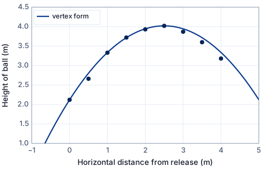
The highest data point, point 6, is taken as the turning (vertex) point: (h, k) = (2.5, 4.02). In vertex (completed-square) form:
y = a(x − 2.5)² + 4.02
A data point is only an estimate of the true turning point; the real maximum or minimum may lie between readings. Say so, and consider refining it (step 5).
Step 2 · Find a from one more point
Substitute point 1, (0, 2.12), far from the vertex:
2.12 = a(0 − 2.5)² + 4.02
a = (2.12 − 4.02) / (−2.5)² = −1.9 / 6.25 = −0.3040
Step 3 · The model in vertex form
y = −0.3040(x − 2.5)² + 4.02
a < 0, so the parabola opens downwards (∩) with a maximum at (2.5, 4.02); the axis of symmetry is x = 2.5.
Step 4 · Convert to y = ax² + bx + c
Expand: a(x − h)² + k = ax² − 2ah·x + (ah² + k), so
b = −2ah = −2 × (−0.3040) × 2.5 = 1.520, c = ah² + k = 2.120
y = −0.3040x² + 1.520x + 2.120
Step 5 · Residuals and goodness of fit
For each point, the residual is the observed value minus the model's value: e = y − ŷ.
| i | x | y (data) | ŷ (model) | y − ŷ | (y − ŷ)² |
|---|---|---|---|---|---|
| 1 | 0 | 2.12 | 2.120 | 0.00 | 0.00 |
| 2 | 0.5 | 2.66 | 2.804 | −0.144 | 0.0207 |
| 3 | 1 | 3.33 | 3.336 | −0.00600 | 0.0000360 |
| 4 | 1.5 | 3.72 | 3.716 | 0.00400 | 0.0000160 |
| 5 | 2 | 3.93 | 3.944 | −0.0140 | 0.000196 |
| 6 | 2.5 | 4.02 | 4.020 | 0.00 | 0.00 |
| 7 | 3 | 3.87 | 3.944 | −0.0740 | 0.00548 |
| 8 | 3.5 | 3.6 | 3.716 | −0.116 | 0.0135 |
| 9 | 4 | 3.18 | 3.336 | −0.156 | 0.0243 |
| Σ | 0.06425 |
- Sum of squared residuals: SSR = Σ(y − ŷ)² = 0.06425
- Total sum of squares about the mean ȳ = 3.381: SST = Σ(y − ȳ)² = 3.265
- Coefficient of determination: R² = 1 − SSR/SST = 1 − 0.06425/3.265 = 0.9803
- Root-mean-square error: RMSE = √(SSR/n) = 0.0845 — a typical size of a residual, in the units of y.
Only two points were used, so this model depends heavily on them. Changing the second point, or nudging the vertex to reduce SSR, is a good piece of reflection (Criterion D).
Method 3: quadratic regression (least squares)
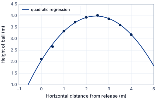
Regression uses all nine points: it chooses a, b and c to minimise the sum of squared residuals. The sums and the three normal equations are shown so you can see what the calculator solves.
Step 1 · Tabulate the sums
| i | x | y | x² | x³ | x⁴ | xy | x²y |
|---|---|---|---|---|---|---|---|
| 1 | 0 | 2.12 | 0 | 0 | 0 | 0 | 0 |
| 2 | 0.5 | 2.66 | 0.25 | 0.125 | 0.0625 | 1.33 | 0.665 |
| 3 | 1 | 3.33 | 1 | 1 | 1 | 3.33 | 3.33 |
| 4 | 1.5 | 3.72 | 2.25 | 3.375 | 5.0625 | 5.58 | 8.37 |
| 5 | 2 | 3.93 | 4 | 8 | 16 | 7.86 | 15.72 |
| 6 | 2.5 | 4.02 | 6.25 | 15.625 | 39.0625 | 10.05 | 25.125 |
| 7 | 3 | 3.87 | 9 | 27 | 81 | 11.61 | 34.83 |
| 8 | 3.5 | 3.6 | 12.25 | 42.875 | 150.0625 | 12.6 | 44.1 |
| 9 | 4 | 3.18 | 16 | 64 | 256 | 12.72 | 50.88 |
| Σ | 18 | 30.43 | 51 | 162 | 548.25 | 65.08 | 183.02 |
n = 9.
Step 2 · The normal equations
Least squares chooses a, b, c to make SSR = Σ(y − ax² − bx − c)² as small as possible. Setting the partial derivatives of SSR to zero gives three linear equations:
- 548.25a + 162b + 51c = 183.02 (Σx⁴, Σx³, Σx², Σx²y)
- 162a + 51b + 18c = 65.08 (Σx³, Σx², Σx, Σxy)
- 51a + 18b + 9c = 30.43 (Σx², Σx, n, Σy)
HL students can derive these by differentiating SSR with respect to each parameter; at SL it is enough to say the calculator minimises SSR.
Step 3 · Solve (matrix or GDC)
Solving the 3 × 3 system (with a matrix inverse, the simultaneous-equation solver, or directly with quadratic regression):
a = −0.3271, b = 1.590, c = 2.055
y = −0.3271x² + 1.590x + 2.055
Turning point: x = −b/(2a) = 2.430, y = 3.987.
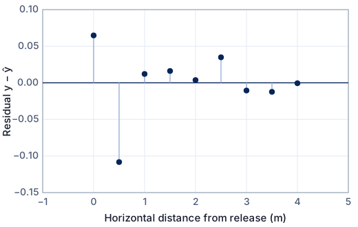
Step 4 · Residuals and goodness of fit
For each point, the residual is the observed value minus the model's value: e = y − ŷ.
| i | x | y (data) | ŷ (model) | y − ŷ | (y − ŷ)² |
|---|---|---|---|---|---|
| 1 | 0 | 2.12 | 2.055 | 0.0648 | 0.00420 |
| 2 | 0.5 | 2.66 | 2.768 | −0.108 | 0.0117 |
| 3 | 1 | 3.33 | 3.318 | 0.0122 | 0.000148 |
| 4 | 1.5 | 3.72 | 3.704 | 0.0162 | 0.000261 |
| 5 | 2 | 3.93 | 3.926 | 0.00372 | 0.0000139 |
| 6 | 2.5 | 4.02 | 3.985 | 0.0348 | 0.00121 |
| 7 | 3 | 3.87 | 3.881 | −0.0105 | 0.000110 |
| 8 | 3.5 | 3.6 | 3.612 | −0.0123 | 0.000151 |
| 9 | 4 | 3.18 | 3.181 | −0.000545 | 0.000000298 |
| Σ | 0.01783 |
- Sum of squared residuals: SSR = Σ(y − ŷ)² = 0.01783
- Total sum of squares about the mean ȳ = 3.381: SST = Σ(y − ȳ)² = 3.265
- Coefficient of determination: R² = 1 − SSR/SST = 1 − 0.01783/3.265 = 0.9945
- Root-mean-square error: RMSE = √(SSR/n) = 0.0445 — a typical size of a residual, in the units of y.
For a quadratic, quote R² (not r, which measures linear correlation only).
Comparing the methods
| Method | Parameters | SSR | R² | RMSE |
|---|---|---|---|---|
| three points and simultaneous equations | 3 | 0.02497 | 0.9923 | 0.0527 |
| vertex form by completing the square | 3 | 0.06425 | 0.9803 | 0.0845 |
| quadratic regression (least squares) | 3 | 0.01783 | 0.9945 | 0.0445 |
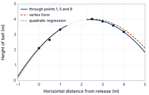
Least squares gives the smallest SSR of any curve of its type, because that is what it minimises. A model through chosen points depends on which points you choose; test that by choosing others. For a fair comparison between different types, also compare the number of parameters and the shape beyond the data — see choosing and comparing models.
What the model tells you
- a = −0.327 < 0: the path is ∩-shaped, as gravity predicts. With constant horizontal speed, a depends on g and the launch speed, which a physics-minded student could use as a check.
- The turning point (2.43, 3.99) is the ball's highest point: it peaks about 2.4 m from release at a height of about 3.99 m.
- Domain: 0 m ≤ x ≤ 4 m (from release to where the ball was last seen). Outside it, the model is not the ball's path.
The same on a GDC
Enter and plot the data first, then fit. The key sequences are for current operating systems; menus differ slightly between versions.
TI-84 Plus CE
- Data: [stat] → 1: Edit… Type the x values in L1 and the y values in L2. To plot: [2nd] [y=] (STAT PLOT) → Plot1: On, Type: scatter, Xlist: L1, Ylist: L2, then [zoom] → 9: ZoomStat.
- Three-point system: APPS → PlySmlt2 → SIMULT EQN SOLVER, 3 equations, 3 unknowns; type the coefficients of a, b, c and the right-hand sides, then SOLVE.
- Or with matrices: [2nd] [x⁻¹] (MATRIX) → EDIT → [A] 3×3 (the x², x, 1 columns) and [B] 3×1 (the y values), then on the home screen [A]⁻¹[B].
- Quadratic regression: [stat] → CALC → 5: QuadReg, Xlist L1, Ylist L2, Store RegEQ Y1. It shows a, b, c and R².
TI-Nspire CX
- Data: Add a Lists & Spreadsheet page; name column A xs and column B ys and type the data. Add a Data & Statistics page (or a Graphs page with menu → Graph Entry/Edit → Scatter Plot) and choose xs and ys.
- Three-point system: Calculator page → menu → Algebra → Solve System of Equations → Solve System of Linear Equations: 3 equations, variables a, b, c.
- Or matrices: type [x1² x1 1; x2² x2 1; x3² x3 1]⁻¹·[y1; y2; y3].
- Regression: menu → Statistics → Stat Calculations → Quadratic Regression, X List xs, Y List ys, save to f1.
Casio fx-CG50
- Data: [MENU] → Statistics. Type the x values in List 1 and the y values in List 2. To plot: [F1] (GRAPH) → [F6] (SET): Graph Type Scatter, XList List1, YList List2; [EXIT], then [F1] (GRAPH1).
- Three-point system: [MENU] → Equation → [F1] (Simultaneous) → [F2] (3 unknowns); type the coefficients; [F1] (SOLVE).
- Or [MENU] → Run-Matrix → [F1] (►MAT) to enter Mat A (3×3) and Mat B (3×1), then Mat A⁻¹ × Mat B.
- Regression: Statistics → [F2] (CALC) → [F3] (REG) → [F3] (X²). It shows a, b, c and R².
In Desmos
Free at desmos.com/calculator. In a regression, ~ means “fit this model”; subscripts are typed with an underscore (x_1 shows as x₁).
- Data in a table with columns x₁, y₁.
- Regression:
y_1 ~ a x_1^2 + b x_1 + c. - Vertex form with a known turning point:
y_1 ~ a (x_1 - 2.5)^2 + 4.02— only a is fitted. - Through three points: type the three equations with sliders, or solve them by hand and type the result to check it passes through the points.
More on technology in the IA: using Desmos, GeoGebra and Excel.
How to write it up in your IA
- Explain why a quadratic suits the context (for a projectile, constant acceleration) before fitting.
- Show the three-point elimination in full once — it is easy to follow and shows algebra — and say why those three points were chosen.
- Show completing the square step by step, and interpret the turning point in context.
- State which points each method uses: three, two, or all of them. That is the heart of the comparison.
- Compare the three models with SSR in one table and explain why regression gives the smallest SSR (it is designed to).
- Reflect: how sensitive are the three-point and vertex models to the points chosen? Try another set and report the change.
These are the points to cover, not sentences to copy. Write every explanation in your own words, about your own data.
Common mistakes
- Choosing three points bunched together: tiny measurement errors then swing the curve wildly.
- Using rounded a and b to find c (carry full values or store them in the calculator).
- Sign slips in completing the square: (x − h)² has the turning point at x = +h.
- Treating the highest data point as the exact vertex without comment.
- Quoting r for a quadratic: use R² (or SSR).
Is this good enough for Criterion E?
- The shape and the context both justify a quadratic.
- At least one method is shown by hand (elimination or completing the square), with technology stated for the rest.
- The turning point is found and interpreted in context.
- Models from different methods are compared with SSR (or R²), and the choice is explained.
- The domain is stated and extrapolation is discussed.
- HL: the normal equations are derived by minimising SSR (partial derivatives), or the 3 × 3 system is solved with matrices and its conditioning discussed.
SL or HL? Criterion E asks for mathematics that fits your course. At SL, fitting with technology is fine when you explain the method and justify every choice. At HL, show more of the mathematics yourself — the last item in the list is an example. See Criterion E and Criterion D.
Frequently asked questions
Which three points should I use to fit a quadratic?
Points spread across the whole data set — typically the first, one near the middle (ideally near the turning point) and the last. Then say how the model changes if you choose different points: that is good reflection.
Is completing the square enough maths for an IA?
On its own it is standard SL content. It becomes strong Criterion E work when it is used for a reason (finding and interpreting the turning point), done correctly and compared with other methods such as regression.
Free: the IA checklist an examiner uses
Every check for Criteria A–E in a 4-page PDF, the mistakes that cost the most marks and a self-assessment grid. We'll email it with a short IA tip every few days, timed to your deadline if you give it. Free — no account, no payment.
While you wait for the email: read the full modelling workflow →