IA modelling, step by step · Power

Power model, step by step: y = a·xⁿ with a log–log plot

AA SLAA HLAI SLAI HL

When y is proportional to a power of x — area and length, period and length, metabolic rate and mass — plot ln y against ln x. A straight line means a power law: its gradient is the power n and its intercept is ln a.

Guidance based on the checklist Pete Bromfield — an IB examiner and former Head of Maths — uses with his own students. Not affiliated with or endorsed by the IB.

Example data, invented for this guide. The context is realistic, but the numbers were made up to show the method. Use your own measured or sourced data in your IA.

When to use it

The shape of the data

The curve passes through (or heads towards) the origin, with no asymptote other than the axes.
Multiplying x by a fixed factor multiplies y by a fixed factor.
ln y against ln x is close to straight.

The context

Physics laws with a power: pendulum period (n = ½), gravity (n = −2), falling distance (n = 2).
Scaling in biology and geometry: surface area, volume, mass.
Anything where theory suggests y ∝ xⁿ and you want to test n.

Course fit: AI SL (models of the form axⁿ), AI HL (log–log linearisation); AA through the laws of logarithms. Comparing the fitted power with a theoretical one is strong at any level.

The example data

A student times 10 swings of a pendulum for several string lengths and divides by 10 to get the period.

Example data: period and length of pendulum
i	x: Length of pendulum (m)	y: Period (s)
1	0.2	0.9
2	0.35	1.18
3	0.5	1.43
4	0.65	1.61
5	0.8	1.8
6	1	2
7	1.2	2.21

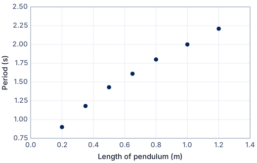
Scatter graph of period against length of pendulum for the example data — Step 1 of any modelling IA: plot the data and describe the shape before fitting anything.

The method: log–log line, then back-substitute

Take natural logs of both variables, fit the least-squares line to (ln x, ln y), and read off n (gradient) and a = e^(intercept). Then refine by least squares in the original units.

Step 1 · Linearise with a log–log plot

If y = axⁿ, taking natural logs gives ln y = n ln x + ln a: a straight line in (ln x, ln y) with gradient n and intercept ln a.

Step 2 · Tabulate the sums

Sums for the least-squares line
i	ln x	ln y	(ln x)²	(ln x)(ln y)	(ln y)²
1	−1.6094	−0.10536	2.5903	0.16957	0.011101
2	−1.0498	0.16551	1.1021	−0.17376	0.027395
3	−0.69315	0.35767	0.48045	−0.24792	0.12793
4	−0.43078	0.47623	0.18557	−0.20515	0.22680
5	−0.22314	0.58779	0.049793	−0.13116	0.34549
6	0	0.69315	0	0.0000	0.48045
7	0.18232	0.79299	0.033241	0.14458	0.62884
Σ	−3.82401	2.96799	4.44148	−0.443845	1.84801

n = 7 points. The transformed values are rounded here; keep them unrounded in your calculator or spreadsheet.

Step 3 · Gradient

m = (nΣXY − ΣX ΣY) / (nΣX² − (ΣX)²)

m = (7 × (−0.443845) − (−3.82401) × 2.96799) / (7 × 4.44148 − (−3.82401)²) = 8.24271 / 16.4673 = 0.5006

Here X = ln x and Y = ln y.

Step 4 · Intercept

X̄ = ΣX/n = −0.54629, Ȳ = ΣY/n = 0.42400

c = Ȳ − m X̄ = 0.42400 − 0.5006 × (−0.54629) = 0.6974

The line of best fit always passes through the mean point (X̄, Ȳ).

Step 5 · Correlation

r = (nΣXY − ΣX ΣY) / √[(nΣX² − (ΣX)²)(nΣY² − (ΣY)²)] = 8.24271 / √(16.4673 × 4.12711) = 0.9999

r² = 0.9997: a very strong positive linear correlation between ln x and ln y.

Step 6 · Back-substitute

n = gradient = 0.5006; ln a = intercept = 0.6974, so a = e^0.6974 = 2.009.

y = 2.009x^0.5006

If a theory predicts the power (for example n = ½ or −2), compare your n with it — that comparison is strong reflection.

Step 7 · Residuals and goodness of fit (in the original units)

For each point, the residual is the observed value minus the model's value: e = y − ŷ.

Residuals
i	x	y (data)	ŷ (model)	y − ŷ	(y − ŷ)²
1	0.2	0.9	0.8975	0.00252	0.00000634
2	0.35	1.18	1.188	−0.00762	0.0000581
3	0.5	1.43	1.420	0.0102	0.000105
4	0.65	1.61	1.619	−0.00901	0.0000812
5	0.8	1.8	1.796	0.00367	0.0000134
6	1	2	2.009	−0.00861	0.0000741
7	1.2	2.21	2.201	0.00946	0.0000894
Σ					0.0004275

Sum of squared residuals: SSR = Σ(y − ŷ)² = 0.0004275
Total sum of squares about the mean ȳ = 1.590: SST = Σ(y − ȳ)² = 1.267
Coefficient of determination: R² = 1 − SSR/SST = 1 − 0.0004275/1.267 = 0.9997
Root-mean-square error: RMSE = √(SSR/n) = 0.00781 — a typical size of a residual, in the units of y.

Step 8 · Refine: least squares on the original data

The log–log line minimises errors in ln y. Minimising SSR in the original units instead (iteratively, from the values above) gives

y = 2.010x^0.5019

GDC power regression gives the log–log answer; Desmos gives this one unless “log mode” is on.

Step 9 · Residuals of the refined model

For each point, the residual is the observed value minus the model's value: e = y − ŷ.

Residuals
i	x	y (data)	ŷ (model)	y − ŷ	(y − ŷ)²
1	0.2	0.9	0.8961	0.00394	0.0000155
2	0.35	1.18	1.187	−0.00661	0.0000437
3	0.5	1.43	1.419	0.0108	0.000116
4	0.65	1.61	1.619	−0.00895	0.0000801
5	0.8	1.8	1.797	0.00324	0.0000105
6	1	2	2.010	−0.00967	0.0000935
7	1.2	2.21	2.202	0.00777	0.0000603
Σ					0.0004200

Sum of squared residuals: SSR = Σ(y − ŷ)² = 0.0004200
Total sum of squares about the mean ȳ = 1.590: SST = Σ(y − ȳ)² = 1.267
Coefficient of determination: R² = 1 − SSR/SST = 1 − 0.0004200/1.267 = 0.9997
Root-mean-square error: RMSE = √(SSR/n) = 0.00775 — a typical size of a residual, in the units of y.

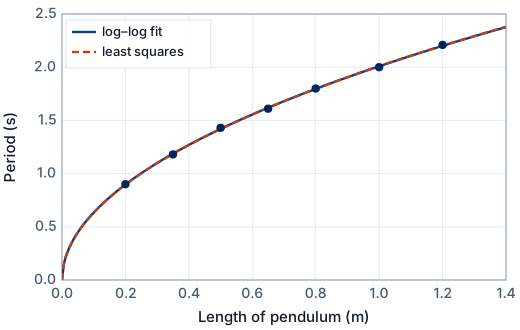
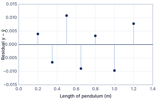
Graph of the data with the fitted power (log–log fit) — Log–log line, then back-substitute: the fitted curves over the example data.

Residual plot for the power fitted to the example data — Residuals against x. Look for a pattern: random scatter about 0 means the model has captured the shape; a curve or a trend means it has not.

What the model tells you

n ≈ 0.501: the period is proportional to the square root of the length, as the simple pendulum formula T = 2π√(L/g) predicts (n = ½).
a ≈ 2.01, and theory says a = 2π/√g, so g = 4π²/a² ≈ 9.79 m s⁻² — close to the accepted 9.81 m s⁻². That is validation against independent knowledge.
Domain: 0.2 m ≤ L ≤ 1.2 m, and small swings. For large swings the formula is less accurate.

The same on a GDC

Enter and plot the data first, then fit. The key sequences are for current operating systems; menus differ slightly between versions.

TI-84 Plus CE

Data: [stat] → 1: Edit… Type the x values in L1 and the y values in L2. To plot: [2nd] [y=] (STAT PLOT) → Plot1: On, Type: scatter, Xlist: L1, Ylist: L2, then [zoom] → 9: ZoomStat.
[stat] → CALC → A: PwrReg, Xlist L1, Ylist L2, Store RegEQ Y1. Result y = a·xᵇ (b is our n).
To show the log–log line: L3 = ln(L1), L4 = ln(L2), LinReg(ax+b) L3, L4.

TI-Nspire CX

Data: Add a Lists & Spreadsheet page; name column A xs and column B ys and type the data. Add a Data & Statistics page (or a Graphs page with menu → Graph Entry/Edit → Scatter Plot) and choose xs and ys.
Power Regression with xs, ys: y = a·xᵇ.
Or columns lnx := ln(xs), lny := ln(ys) and Linear Regression.

Casio fx-CG50

Data: [MENU] → Statistics. Type the x values in List 1 and the y values in List 2. To plot: [F1] (GRAPH) → [F6] (SET): Graph Type Scatter, XList List1, YList List2; [EXIT], then [F1] (GRAPH1).
Statistics → [F2] (CALC) → [F3] (REG) → [F6] (▷) → [F3] (Pwr): y = a·xᵇ.

In Desmos

Free at desmos.com/calculator. In a regression, ~ means “fit this model”; subscripts are typed with an underscore (x_1 shows as x₁).

Data in x₁, y₁.
y_1 ~ a x_1^n (direct least squares; log mode reproduces the GDC).
To show the log–log line: a table with columns ln(x_1), ln(y_1) and Y ~ m X + c.

More on technology in the IA: using Desmos, GeoGebra and Excel.

How to write it up in your IA

Say what power theory predicts before fitting, if there is one.
Show the log–log table and graph; explain why a straight line there means a power law (laws of logs).
Find n and a from the line and back-substitute.
Compare the fitted n with theory and use a to estimate a physical constant if possible.
Mention the difference between the log–log fit and direct least squares.

These are the points to cover, not sentences to copy. Write every explanation in your own words, about your own data.

Common mistakes

Confusing a power model (x is the base) with an exponential model (x is the exponent).
Using a log–log plot with x ≤ 0 or y ≤ 0.
Rounding n to the theoretical value before checking whether the data support it.

Is this good enough for Criterion E?

The power form is justified by context or by the log–log plot.
n and a are found from the log–log line with the transformation explained.
The fitted n is compared with theory (if any) and its meaning explained.
The fit is checked with residuals in the original units.
HL: the uncertainty in n is discussed (for example, the effect of timing errors), or the model is derived from dimensional analysis.

SL or HL? Criterion E asks for mathematics that fits your course. At SL, fitting with technology is fine when you explain the method and justify every choice. At HL, show more of the mathematics yourself — the last item in the list is an example. See Criterion E and Criterion D.

Frequently asked questions

How can I tell a power model from an exponential model?

Plot both linearisations: ln y against ln x (straight for a power model) and ln y against x (straight for an exponential). Whichever is straighter, with residuals showing no pattern, is the better candidate.

Free: the IA checklist an examiner uses

Every check for Criteria A–E in a 4-page PDF, the mistakes that cost the most marks and a self-assessment grid. We'll email it with a short IA tip every few days, timed to your deadline if you give it. Free — no account, no payment.

Get the free checklist