Log–log plot and power regression: linearise your data
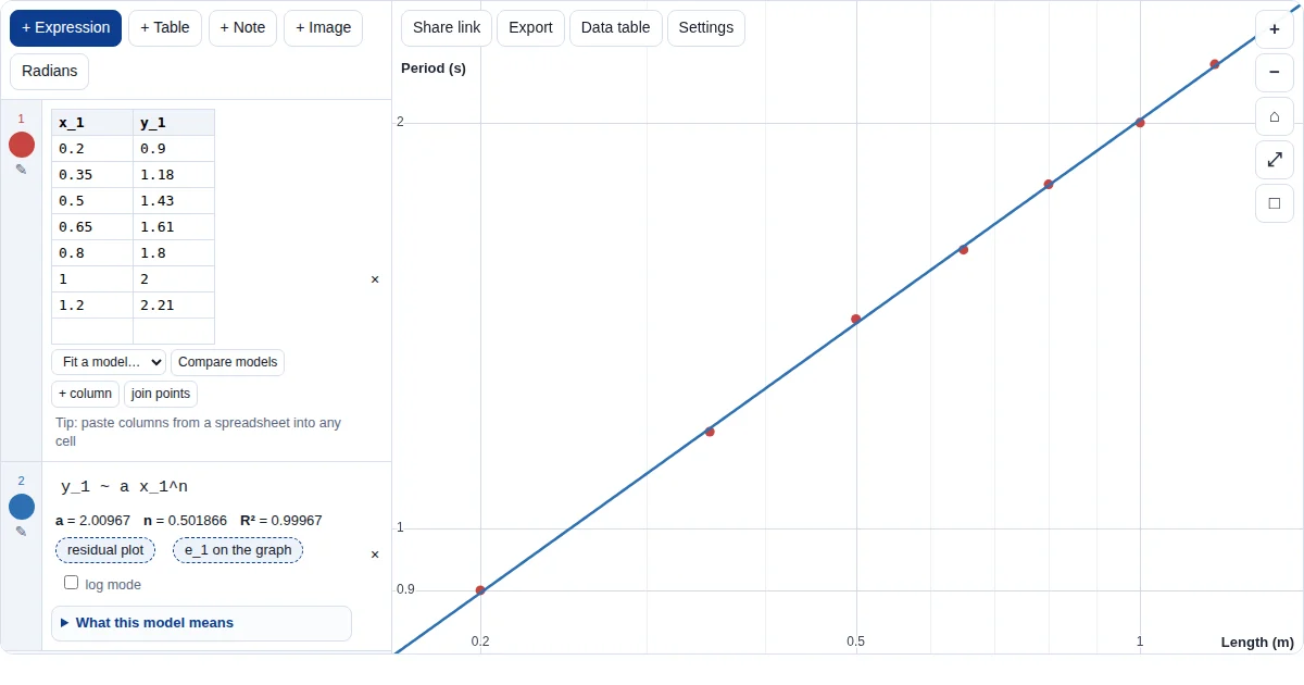
If y = axⁿ, then log y = n log x + log a: on log–log axes a power law is a straight line with gradient n. The Grapher draws log axes and fits the power model for you.
How to do it
- Enter your data. Paste or type the table. Log axes need positive values.
- Fit the power model. Type
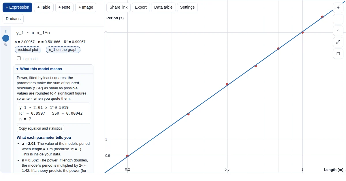
y_1 ~ a x_1^n. The Grapher shows a, n and R². - Switch to log axes. In the model's What this model means panel press Linearise it, or turn on log scales for x and y in Settings. Power data lie on a straight line on log–log axes; exponential data on a log y-axis only; logarithmic data on a log x-axis only.
- Read the gradient. On log–log axes the gradient of the line is n and the intercept is log a, which is how the model is linearised by hand.
Good to know
- Which axes straighten which model: log–log for y = axⁿ, log y for y = ae^(kx), log x for y = a ln x + b.
- Ticks on log axes are at 1, 2 and 5 × 10ⁿ, so you can still read values off the graph.
- A GDC's power regression fits ln y against ln x; turn on log mode under the fit to get the same answer.
Frequently asked questions
What is a log–log plot?
A graph with logarithmic scales on both axes. A power law y = axⁿ becomes the straight line log y = n log x + log a, so the gradient is n.
How do I linearise data?
Fit the model, open “What this model means” and press “Linearise it”: the Grapher switches on the log axes that make that model a straight line. You can also turn the log scales on yourself in Settings.
Can I do a semi-log plot?
Yes: turn on the log scale for y only (for exponential data) or for x only (for logarithmic data) in Settings.
Learn more
- Power model, worked
- Exponential model, worked
- Exponent and logarithm laws (AA SL notes)
- Choosing and comparing models
- IA modelling, step by step
More Grapher guides
The Grapher is our own free tool (graph.mathrevision.co.uk), built for IB, A Level and IGCSE students. It is not an exam calculator: practise on your own GDC for calculator papers.