Free IB Maths AI HL lesson: Non-linear regression & residual analysis
A ready-to-teach IB Maths AI HL lesson on Non-linear regression & residual analysis (Unit 2 · Functions): editable slides and teacher notes, free; a printable worksheet in 3 levels with answers for school plans. About 55 minutes.
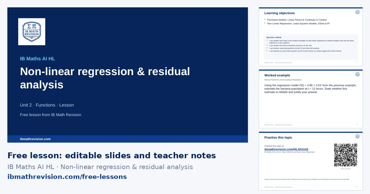
Free with a teacher account. Sign in with Google, Microsoft or email and download the slides and teacher notes.
What's inside
- Slides (PowerPoint, editable) · freeabout 12 slides: do now, objectives, key ideas, a worked example step by step, “your turn”, practice QR code, exit ticket
- Teacher notes (PDF) · freelesson plan with timings, common mistakes, homework links
- Worksheet (PDF) · school plans6 questions, 32 marks: Fluency, Reasoning, Exam-style. Included with school plans and the teacher trial.
- Answers (PDF) · school plansthe answer to every worksheet question, from its mark scheme. Included with school plans and the teacher trial.
Learning objectives
- Piecewise Models: Linear Pieces & Continuity in Context
- Non-Linear Regression: Least-Squares Models, SSres & R²
Key ideas on the slides
- Choose a model from the shape of the data and the context: linear (constant rate), quadratic (one turning point), exponential (constant percentage change), power y = axⁿ (variation), sinusoidal (periodic), logistic (growth with a limit).
- Fit the model with the matching regression on the GDC; write the equation with the parameters to 3 s.f.
- Judge the fit: R² (or r for a linear model) close to 1 means a good fit; the sum of squared residuals SSᵣₑₛ is smaller for a better fit.
- Check the model makes sense beyond the data (e.g. exponential growth cannot continue forever) and state a limitation.
By the end of the lesson, students should be able to answer a question like: A dataset of population vs. year is modelled with a cubic regression. Plot the residuals and comment on whether the cubic model is appropriate.
Key vocabulary
- model: A function used to describe a real situation.
- residual: The observed value minus the value predicted by the model.
- coefficient of determination: R²: the proportion of the variation in y explained by the model.
- regression line: The line of best fit that minimises the sum of squared vertical distances.
- interpolation: Predicting within the range of the data.
Common mistakes this lesson tackles
- Modelling: regression on the GDC, r² for non-linear models, context of the variable. Use the GDC's regression for the model named. Compare non-linear fits with R² and quote both values. Define the variable ("t = years after 2010") before substituting, and answer the comparison the question actually asks.
- Choosing a model only from R² without looking at the context or the graph.
- Using r to judge a non-linear model.
- Extrapolating far beyond the data.
The worked example
Using the regression model P(t) = 4.88 × 3.01ᵗ from the previous example, estimate the bacteria population at t = 12 hours. State whether this estimate is reliable and justify your answer.
- Substitute t = 12 into the exponential model: P(12) = 4.88 × 3.01¹².
- Evaluate using the GDC: P(12) ≈ 2 666 285.
- State the estimate: The estimated population is 2 670 000 bacteria (to 3 s.f.).
- Analyse the reliability based on the original data range (t=1 to t=4).
- Conclude: The estimate is not reliable.
- Justify: It relies heavily on extrapolation far outside the known data range, and exponential growth models rarely continue indefinitely in reality due to limiting factors like space and resources.
Tip: Estimates made via extrapolation are inherently unreliable. Even if a model has an R² value of 1.00 inside the data range, you must state that extrapolating outside the domain renders the prediction untrustworthy.
Calculator tips
- STAT → regression: LinReg, QuadReg, CubicReg, ExpReg, PwrReg, SinReg or Logistic; turn on diagnostics to see r and R².
- LinReg(a+bx) on the GDC; store the equation to evaluate predictions.
Where this lesson fits
Non-linear regression & residual analysis is in Unit 2 · Functions of the IB Maths AI HL scheme of work.
- The lesson before: Combined transformations (scheme-of-work lessons: Transformations of graphs)
- The next lesson: Domain, range, composite & inverse functions (scheme-of-work lessons: Function Features: Domain, Range & Asymptotes with Technology; Asymptotes, Intercepts & Domain in Context; Composite & Inverse Functions: (f∘g)(x), f⁻¹(x) & Domain Restriction)
Lesson plan
| 0–5 min | Do now: students write down what they remember about Combined transformations and Vertical + horizontal stretches |
| 5–8 min | Share the learning objective and success criteria |
| 8–20 min | Teach: the worked example, step by step; students copy the method |
| 20–25 min | Your turn: 1 mini-whiteboard question; check every board before moving on |
| 25–42 min | Practise: the worksheet (6 questions in 3 levels, with school plans and the teacher trial) or the topic's practice questions online; move up a level after two right in a row |
| 42–47 min | Plenary: 1-question exit ticket; collect it to plan the next lesson |
For students: practise this topic
The worksheet's QR code opens the IB Maths AI HL Unit 2: Data Collection and Non-Linear Regression practice questions.
With a school plan
Set Non-linear regression & residual analysis as homework marked by AI, print this lesson's levelled worksheet with answers, and rebuild the lesson for your class with Create lesson. Free for 30 days as a teacher, no card.
Is it free, can I edit the slides, what do students use for homework? See questions teachers ask.