Free IB Maths AI HL lesson: Normal distribution
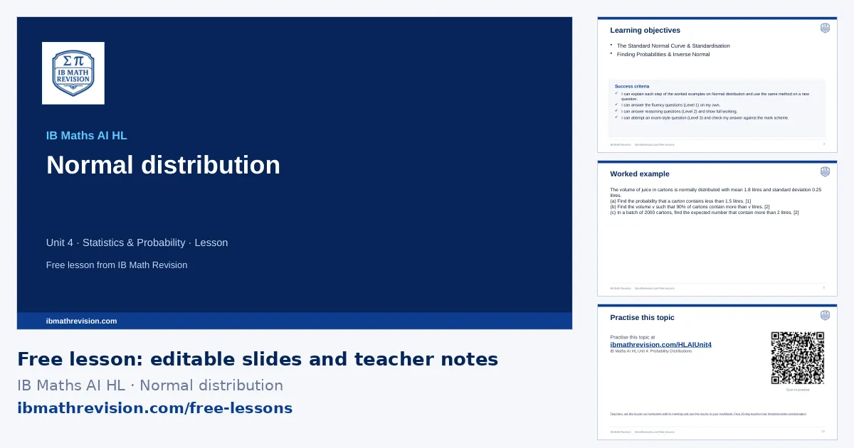
A ready-to-teach IB Maths AI HL lesson on Normal distribution (Unit 4 · Statistics & Probability): editable slides and teacher notes, free; a printable worksheet in 3 levels with answers for school plans. About 55 minutes.
Free with a teacher account. Sign in with Google, Microsoft or email and download the slides and teacher notes.
What's inside
- Slides (PowerPoint, editable) · freeabout 12 slides: do now, objectives, key ideas, a worked example step by step, “your turn”, practice QR code, exit ticket
- Teacher notes (PDF) · freelesson plan with timings, common mistakes, homework links
- Worksheet (PDF) · school plans6 questions, 27 marks: Fluency, Reasoning, Exam-style. Included with school plans and the teacher trial.
- Answers (PDF) · school plansthe answer to every worksheet question, from its mark scheme. Included with school plans and the teacher trial.
Learning objectives
- The Standard Normal Curve & Standardisation
- Finding Probabilities & Inverse Normal
Key ideas on the slides
- X ~ N(μ, σ²) is continuous, symmetric about μ, bell-shaped; about 68%, 95% and 99.7% of values lie within 1, 2 and 3 standard deviations of the mean.
- For a continuous distribution P(X = a) = 0, so P(X < a) = P(X ≤ a).
- Sketch the curve and shade the region before using the GDC; symmetry helps: P(X > μ + k) = P(X < μ − k).
- Inverse normal: given an area, find the boundary value (use the left-tail area).
By the end of the lesson, students should be able to answer a question like: If X~N(50, 25), find the probability that X is greater than 55.
Key vocabulary
- normal distribution: A symmetric, bell-shaped continuous distribution.
- mean: μ, the centre of the curve.
- standard deviation: σ, the spread; note N(μ, σ²) gives the variance.
Common mistakes this lesson tackles
- Distributions: variances add, the normal is continuous, the binomial coefficient. For independent X and Y: Var(X ± Y) = Var(X) + Var(Y); Var(aX) = a²Var(X). State the final distribution, e.g. X − Y ~ N(20, 25), before finding probabilities.
- Using σ² as σ (the second parameter is the variance).
- Using the right-tail area in inverse normal without converting it.
- Rounding μ or σ in the middle of a question.
Calculator tips
- normalcdf(lower, upper, μ, σ) and invNorm(area, μ, σ) (left tail).
Where this lesson fits
Normal distribution is in Unit 4 · Statistics & Probability of the IB Maths AI HL scheme of work.
- The lesson before: Poisson distribution (scheme-of-work lessons: Modelling Random Events in Time or Space; Calculating Probabilities with the GDC; Poisson Revisited: Sums of Independent Poisson Variables)
- The next lesson: Exponential distribution (extension) (scheme-of-work lessons: Continuous random variables)
Lesson plan
| 0–5 min | Do now: students write down what they remember about Poisson distribution and Binomial distribution |
| 5–8 min | Share the learning objective and success criteria |
| 8–20 min | Teach: the worked example, step by step; students copy the method |
| 20–25 min | Your turn: 1 mini-whiteboard question; check every board before moving on |
| 25–42 min | Practise: the worksheet (6 questions in 3 levels, with school plans and the teacher trial) or the topic's practice questions online; move up a level after two right in a row |
| 42–47 min | Plenary: 1-question exit ticket; collect it to plan the next lesson |
For students: practise this topic
The worksheet's QR code opens the IB Maths AI HL Unit 4: Probability Distributions practice questions.
With a school plan
Set Normal distribution as homework marked by AI, print this lesson's levelled worksheet with answers, and rebuild the lesson for your class with Create lesson. Free for 30 days as a teacher, no card.
Is it free, can I edit the slides, what do students use for homework? See questions teachers ask.